15 Multiple Regression
15.1 Fitting regression with categorical predictors
In the final weeks of POLS0008 we explored regression using a quantitative explanatory variable. It turns out we can also use regression with categorical explanatory variables. It is quite straightforward to run it. You will need to use your merged file from POLS0008 - Week 8. If you do not have a copy of this file in your working directory, download the election17aps17.csv file from Moodle.
Let’s assume we were interested in percent of votes for a conservative candidate in England compared with Scotland and Wales. There is a variable in our election17aps17 object called country_name. We could collaspe this 3 category variable into a binary variable: England or Wales and Scotland.
election17aps17$england<-election17aps17$country_name #create a new variable called country that replicates the country_name variable
levels(election17aps17$england) <- list(England="England", Other=c("Scotland", "Wales")) # collaspe Scotland and Wales into one level and England into another
summary(election17aps17$england)
#> England   Other
#>     533      99
This is how you would express the model with a categorical explanatory variable. It is exactly the same as you specify a model with a continuous explanatory variable, however, R recognises that country is a factor variables and treats it accordingly. You will need to recreate the con.per variable if you have downloaded a fresh copy of election17aps17 from Moodle.
fit_2 <- lm(con.per ~ england, data=election17aps17)Let’s have a look at the results:
summary(fit_2)
#>
#> Call:
#> lm(formula = con.per ~ england, data = election17aps17)
#>
#> Residuals:
#>     Min      1Q  Median      3Q     Max
#> -0.3765 -0.1060  0.0191  0.1210  0.2496
#>
#> Coefficients:
#>              Estimate Std. Error t value Pr(>|t|)
#> (Intercept)   0.44955    0.00622   72.27   <2e-16 ***
#> englandOther -0.15278    0.01570   -9.73   <2e-16 ***
#> ---
#> Signif. codes:  0 '***' 0.001 '**' 0.01 '*' 0.05 '.' 0.1 ' ' 1
#>
#> Residual standard error: 0.143 on 629 degrees of freedom
#>   (1 observation deleted due to missingness)
#> Multiple R-squared:  0.131,  Adjusted R-squared:  0.129
#> F-statistic: 94.6 on 1 and 629 DF,  p-value: <2e-16
As you will see the output does not look too different compared to the model with a continuous explanatory variable. But notice that in the print out you see how the row with the coefficient and other values for our explanatory variable country we see that R is printing countryOther. What does this mean?
Remember t tests from POLS0008? It turns out that a linear regression model with just one dichotomous/binary categorical predictor is just the equivalent of a two sample t test. When you only have one predictor the value of the intercept is the mean value of the reference category and the coefficient for the slope tells you how much higher (if it is positive) or how much lower (if it is negative) is the mean value for the other category in your factor.
The reference category is the one for which R does not print the level next to the name of the variable for which it gives you the regression coefficient. Here we see that the named level is “Other”. That’s telling you that the reference category here is “England”. Therefore the Y intercept in this case is the mean proportion of people voting conservative in England, whereas the coefficient for the slope is telling you how much lower the percent value is in Wales and Scotland. Don’t believe me?
mean(election17aps17$con.per[election17aps17$england == "England"], na.rm=TRUE)
#> [1] 0.45mean(election17aps17$con.per[election17aps17$england == "England"], na.rm=TRUE) - mean(election17aps17$con.per[election17aps17$england == "Other"], na.rm=TRUE)
#> [1] 0.153So, to reiterate, for a binary predictor in a simple regression model (i.e. a model with only one explanatory variable), the coefficient is nothing else than the difference between the mean of the two levels in your factor variable, between the averages in your two groups.
With categorical variables encoded as factors you always have a situation like this: a reference category and then as many additional coefficients as there are additional levels in your categorical variable. Each of these additional categories is input into the model as “dummy” variables. Here our categorical variable has two levels, thus we have only one dummy variable. There will always be one fewer dummy variable than the number of levels. The level with no dummy variable England in this example — is known as the reference category or the baseline category.
It turns out then that the regression table is printing out for us a t test of statistical significance for every explanatory variable in the model. If we look at the table above this t value is -9.728 and the p value associated with it is near 0. This is indeed considerably lower than the conventional significance level of 0.05. So we could conclude that the probability of obtaining this value if the null hypothesis were true is very low. However, the observed r squared is much lower than a model with only, for example, the Manager variable.
Imagine, however, that you are looking at the relationship between percent voting conservative and region. In our data set region_name has 10 levels that are alphabetically ordered.
levels(election17aps17$region_name)
#>  [1] "East"                     "East Midlands"
#>  [3] "London"                   "North East"
#>  [5] "North West"               "Scotland"
#>  [7] "South East"               "South West"
#>  [9] "Wales"                    "West Midlands"
#> [11] "Yorkshire and The Humber"
If we were to run a regression model this would result in a model with 9 dummy variables. The coefficient of each of these dummies would be telling you how much higher or lower (if the sign were negative) was the percent voting conservative in each region of Great Britain for which you have a dummy compared to your reference category or baseline. One thing that is important to keep in mind is that R by default will use as the baseline category the first level in your factor. Since region has these levels alphabetically ordered that means that your reference category would be “East”. If you want to change this you may need to reorder the levels. One way of doing this in while fitting the regression model is to use the relevel function within your formula call in lm. As a general rule of thumb is it good practice to use the largest group as your reference category. We can find out which region contains the most constituencies by running summary(election17aps17$region_name). We could then run the following model and call for the summary.
fit_3 <- lm(con.per ~ relevel(region_name, "South East"), data=election17aps17)
summary(fit_3)
#>
#> Call:
#> lm(formula = con.per ~ relevel(region_name, "South East"), data = election17aps17)
#>
#> Residuals:
#>     Min      1Q  Median      3Q     Max
#> -0.3818 -0.0815  0.0120  0.0827  0.2935
#>
#> Coefficients:
#>                                                            Estimate
#> (Intercept)                                                 0.54385
#> relevel(region_name, "South East")East                      0.00126
#> relevel(region_name, "South East")East Midlands            -0.04417
#> relevel(region_name, "South East")London                   -0.20793
#> relevel(region_name, "South East")North East               -0.20307
#> relevel(region_name, "South East")North West               -0.18457
#> relevel(region_name, "South East")Scotland                 -0.26771
#> relevel(region_name, "South East")South West               -0.02842
#> relevel(region_name, "South East")Wales                    -0.21664
#> relevel(region_name, "South East")West Midlands            -0.06097
#> relevel(region_name, "South East")Yorkshire and The Humber -0.15063
#>                                                            Std. Error
#> (Intercept)                                                   0.01332
#> relevel(region_name, "South East")East                        0.02077
#> relevel(region_name, "South East")East Midlands               0.02231
#> relevel(region_name, "South East")London                      0.01947
#> relevel(region_name, "South East")North East                  0.02618
#> relevel(region_name, "South East")North West                  0.01933
#> relevel(region_name, "South East")Scotland                    0.02066
#> relevel(region_name, "South East")South West                  0.02110
#> relevel(region_name, "South East")Wales                       0.02336
#> relevel(region_name, "South East")West Midlands               0.02066
#> relevel(region_name, "South East")Yorkshire and The Humber    0.02122
#>                                                            t value
#> (Intercept)                                                  40.83
#> relevel(region_name, "South East")East                        0.06
#> relevel(region_name, "South East")East Midlands              -1.98
#> relevel(region_name, "South East")London                    -10.68
#> relevel(region_name, "South East")North East                 -7.76
#> relevel(region_name, "South East")North West                 -9.55
#> relevel(region_name, "South East")Scotland                  -12.95
#> relevel(region_name, "South East")South West                 -1.35
#> relevel(region_name, "South East")Wales                      -9.27
#> relevel(region_name, "South East")West Midlands              -2.95
#> relevel(region_name, "South East")Yorkshire and The Humber   -7.10
#>                                                            Pr(>|t|)
#> (Intercept)                                                 < 2e-16 ***
#> relevel(region_name, "South East")East                       0.9515
#> relevel(region_name, "South East")East Midlands              0.0481 *
#> relevel(region_name, "South East")London                    < 2e-16 ***
#> relevel(region_name, "South East")North East                3.6e-14 ***
#> relevel(region_name, "South East")North West                < 2e-16 ***
#> relevel(region_name, "South East")Scotland                  < 2e-16 ***
#> relevel(region_name, "South East")South West                 0.1785
#> relevel(region_name, "South East")Wales                     < 2e-16 ***
#> relevel(region_name, "South East")West Midlands              0.0033 **
#> relevel(region_name, "South East")Yorkshire and The Humber  3.4e-12 ***
#> ---
#> Signif. codes:  0 '***' 0.001 '**' 0.01 '*' 0.05 '.' 0.1 ' ' 1
#>
#> Residual standard error: 0.121 on 620 degrees of freedom
#>   (1 observation deleted due to missingness)
#> Multiple R-squared:  0.387,  Adjusted R-squared:  0.377
#> F-statistic: 39.2 on 10 and 620 DF,  p-value: <2e-16
What can you infer about the regional differences in the percent voting conservative compared with the reference category? In which region is the mean percent highest and lowest?
15.2 Motivating to multiple regression
So we have seen our models with just one predictor or explanatory variable. We can build ‘better’ models by expanding the number of predictors (although keep in mind you should also aim to build models as parsimonious as possible).
Another reason why it is important to think about additional variables in your model is to control for spurious correlations (although here you may also want to use your common sense when selecting your variables!). You have heard that correlation does not equal causation. Just because two things are associated we cannot assume that one is the cause for the other. Typically we see how the pilots switch the secure the belt button when there is turbulence. These two things are associated, they tend to come together. But the pilots are not causing the turbulences by pressing a switch! The world is full of spurious correlations, associations between two variables that should not be taking too seriously. You can explore a few here.
Looking only at covariation between pair of variables can be misleading. It may lead you to conclude that a relationship is more important than it really is. This is no trivial matter, but one of the most important ones we confront in research and policy.
It is not an exaggeration to say that most quantitative explanatory research is about trying to control for the presence of confounders, variables that may explain explain away observed associations. Think about any social science question: Are married people less prone to depression? Or is it that people that get married are different from those that don’t (and are there pre-existing differences that are associated with less depression)? Are ethnic minorities more likely to vote for centre-left political parties? Or is it that there are other factors (e.g. socioeconomic status, area of residence, sector of employment) that, once controlled, would mean there is no ethnic group difference in voting? You should be starting to think of these types of research questions for the dissertation.
Multiple regression is one way of checking the relevance of competing explanations. You could set up a model where you try to predict voting behaviour with an indicator of ethnicity and an indicator of structural disadvantage. If after controlling for structural disadvantage you see that the regression coefficient for ethnicity is still significant you may be onto something, particularly if the estimated effect is still large. If, on the other hand, the t test for the regression coefficient of your ethnicity variable is no longer significant, then you may be tempted to think structural disadvantage is a confounder (or mediator, but we’ll leave that term for next year) for vote selection.
15.3 Fitting and interpreting a multiple regression model
It could not be any easier to fit a multiple regression model. You simply modify the formula in the lm() function by adding terms for the additional inputs.
fit_4 <- lm(con.per ~ Manager+england, data=election17aps17)
summary(fit_4)
#>
#> Call:
#> lm(formula = con.per ~ Manager + england, data = election17aps17)
#>
#> Residuals:
#>     Min      1Q  Median      3Q     Max
#> -0.4031 -0.0882  0.0201  0.1027  0.2866
#>
#> Coefficients:
#>              Estimate Std. Error t value Pr(>|t|)
#> (Intercept)    0.2883     0.0163   17.74   <2e-16 ***
#> Manager        0.0149     0.0014   10.67   <2e-16 ***
#> englandOther  -0.1247     0.0146   -8.51   <2e-16 ***
#> ---
#> Signif. codes:  0 '***' 0.001 '**' 0.01 '*' 0.05 '.' 0.1 ' ' 1
#>
#> Residual standard error: 0.131 on 626 degrees of freedom
#>   (3 observations deleted due to missingness)
#> Multiple R-squared:  0.267,  Adjusted R-squared:  0.265
#> F-statistic:  114 on 2 and 626 DF,  p-value: <2e-16
With more than one input, you need to ask yourself whether all of the regression coefficients are zero. This hypothesis is tested with a F test. Here we are assuming the residuals are normally distributed, though with large samples the F statistic approximates the F distribution.
You see the F test printed at the bottom of the summary output and the associated p value, which in this case is way below the conventional .05 that we use to declare statistical significance and reject the null hypothesis. At least one of our explantory variables must be related to our dependent variable.
Notice that the table printed also reports a t test for each of the predictors. These are testing whether each of these predictors is associated with the response variable when adjusting for the other variables in the model. They report the partial effect of adding that variable to the model. In this case we can see that both variables seem to be significantly associated with the dependent variable.
If we look at the r squared we can now see that it is higher than before with either the Manager variable only or the England variable only. R squared will always increase as a consequence of adding new variables, even if the new variables added are weakly related to the response variable. The adjusted R2 avoids this problem because it controls for the number of variables we have included in our model.
We see that the coefficient for Manager changes by about 13% and the coefficient for england reduces by 18%. This suggests that the percent of managerial employed people in a constituency explains some of the difference between England and other countries in Britain combined (i.e. Scotland and Wales).
The interpretation of the two explanatory variable also changes in a multiple regression model. A common interpretation is that now the regression for each variable tells you about changes in Y related to that variable when the other variables in the model are held constant. So, for example, you could say the coefficient for Manager represents the increase in percent of the vote for a conservative candidate for every one-unit increase in the percent of people working in managerial occupations when holding all other variables in the model constant (in this case that refers to holding constant country).
Other interpretations are also possible and are more generalisable. Gelman and Hill (2007: p. 34) emphasise what they call the predictive interpretation that considers how “the outcome variable differs, on average, when comparing two groups of units that differ by 1 in the relevant predictor while being identical in all the other predictors”. So if you’re regressing y on u and v, the coefficient of u is the average difference in y per difference in u, comparing pairs of items that differ in u but are identical in v.
So, for example, in this case we could say that comparing constituencies that have the same percent of people working inmanagerial occupations but that differed in whether they are in England versus Scotland and Wales, the model predits an expected difference of -12.46 in their percent of votes for a conservative candidate. And that constituencies in the same country, but that differ by one point in the percent working in higher managerial occupations, we would expect to see a difference of 1.49 in percent of votes for a conservative candidate. So we are interpreting the regression slopes as comparisons of constituencies that differ in one explanatory variable while being at the same levels of the other explanatory variables.
As you can see, interpreting regression coefficients can be kind of tricky. The relationship between the response y and any one explanatory variable can change greatly depending on what other explanatory variables are present in the model.
For example, if you contrast this model with the one we run with only country as an explanatory variable you will notice the intercept has changed. You cannot longer read the intercept as the mean percent of votes for a conservative candidate in England. Adding predictors to the model changes their meaning. Now the intercept indexes the value percent of votes for a conservative candidate in English constituencies that have 0% working in managerial occupations. You might have noticed that you there are no constituencies that have 0% working in managerial occupations. You can check by using the describeBy function in the psych package. This means there is little worth bothering to interpret the intercept, which is often the case in regression analysis. That does not mean the intercept is redundant, it is essential for you to predict values of y for given values of our x’s.
Something you need to be particularly careful about is to interpret the coefficients in a causal manner. With observational data, regression coefficients should not be read as indexing causal relations. This sort of textbook warning is, however, often neglectfully ignored by professional researchers. Often authors carefully draw sharp distinctions between causal and correlational claims when discussing their data analysis, but then interpret the correlational patterns in a totally causal way in their conclusion section.
Comparing the simple models with this more complex model we could say that adjusting for England does not change much the impact of Managerial in percent voting conservative as vice versa. Neverthelss, there remains a significant statistical effect of england on the percent voting conservative.
15.4 Model building and comparison
How do you construct a good model? This partly depends on your goal, although there are commonalities. You do want to start with theory as a way to select your predictors and when specifying the nature of the relationship to your response variable (e.g., additive, multiplicative). A tempting strategy is to put all variables possible into a regression model and see which are significant. This can cause problems if an irrelevant variable draws strength from a variable (X) that we expect to be related to the outcome variable (Y) but is also correlated with the irrelevant variable. This will make it harder to accurately assign the variance of Y to X, and reducing the precision of the estimates.
We can formally test whether a certain subset of the coefficients are equal to 0 using a partial F-test. This test involves comparing the the sum of squared residuals (RSS) from a reduced model (excluding the parameters we hypothesis are equal to zero) with the SSE from the full model (including all of the parameters).
In R we can perform partial F-tests by fitting both the reduced and full models separately and thereafter comparing them using the anova function.
Suppose we include the variables Manager, england and White in our model and are interested in testing whether White is significant after taking Manager and england into consideration.
reduced = lm(con.per ~ Manager+england, data=election17aps17) # Reduced model
full = lm(con.per ~ Manager+england+White, data=election17aps17) # Full Model
The following code performs the partial F-test:
anova(reduced, full)# Compare the models
#> Analysis of Variance Table
#>
#> Model 1: con.per ~ Manager + england
#> Model 2: con.per ~ Manager + england + White
#>   Res.Df   RSS Df Sum of Sq   F Pr(>F)
#> 1    626 10.81
#> 2    625  7.79  1      3.02 242 <2e-16 ***
#> ---
#> Signif. codes:  0 '***' 0.001 '**' 0.01 '*' 0.05 '.' 0.1 ' ' 1
The output shows the results of the partial F-test. Since F=242.13 (p-value=0.1685) we can reject the null hypothesis that the coefficient for White=0. It would be too time consuming to apply this method for every possible combination of nested models with all of the variables in our dataset (assuming a theorectically relationship between each explanatory variable and our dependent variable). Ideally, we would like to perform variable selection by trying out a lot of different models, each containing a different subset of the predictors. Selecting a subset of predictor variables from a larger set (e.g., stepwise selection) is a controversial topic. You can perform stepwise selection (forward, backward, both) using the stepAIC function from the MASS package. stepAIC() performs stepwise model selection by exact AIC. AIC provides measures of goodness of fit that is often preferred in model selection to the R2. I recommend you only apply stepwise selection methods when you are exploring your data rather than relying on them to provide you with an optimal model.
Let’s try an example where we include a range of other variables that we expect to be related to the percent of votes for a conservative candidate:
library(MASS)
step.model <- lm(con.per ~ Manager+england+White+Admin+British+Public+Employment, data=election17aps17)
summary(step.model)
#>
#> Call:
#> lm(formula = con.per ~ Manager + england + White + Admin + British +
#>     Public + Employment, data = election17aps17)
#>
#> Residuals:
#>     Min      1Q  Median      3Q     Max
#> -0.3298 -0.0637  0.0101  0.0793  0.2662
#>
#> Coefficients:
#>               Estimate Std. Error t value Pr(>|t|)
#> (Intercept)  -3.76e-01   6.00e-02   -6.27  6.8e-10 ***
#> Manager       8.78e-03   1.18e-03    7.44  3.4e-13 ***
#> englandOther -1.42e-01   1.54e-02   -9.25  < 2e-16 ***
#> White         4.43e-03   3.40e-04   13.06  < 2e-16 ***
#> Admin         5.75e-05   1.33e-03    0.04  0.96543
#> British      -4.68e-04   4.85e-04   -0.96  0.33572
#> Public       -4.82e-03   1.36e-03   -3.53  0.00044 ***
#> Employment    6.22e-03   7.59e-04    8.20  1.4e-15 ***
#> ---
#> Signif. codes:  0 '***' 0.001 '**' 0.01 '*' 0.05 '.' 0.1 ' ' 1
#>
#> Residual standard error: 0.103 on 621 degrees of freedom
#>   (3 observations deleted due to missingness)
#> Multiple R-squared:  0.553,  Adjusted R-squared:  0.548
#> F-statistic:  110 on 7 and 621 DF,  p-value: <2e-16
step <- stepAIC(step.model, direction="both")
#> Start:  AIC=-2851
#> con.per ~ Manager + england + White + Admin + British + Public +
#>     Employment
#>
#>              Df Sum of Sq  RSS   AIC
#> - Admin       1     0.000 6.59 -2853
#> - British     1     0.010 6.60 -2852
#> <none>                    6.59 -2851
#> - Public      1     0.133 6.72 -2841
#> - Manager     1     0.587 7.18 -2800
#> - Employment  1     0.714 7.31 -2789
#> - england     1     0.909 7.50 -2772
#> - White       1     1.809 8.40 -2701
#>
#> Step:  AIC=-2853
#> con.per ~ Manager + england + White + British + Public + Employment
#>
#>              Df Sum of Sq  RSS   AIC
#> - British     1     0.010 6.60 -2854
#> <none>                    6.59 -2853
#> + Admin       1     0.000 6.59 -2851
#> - Public      1     0.343 6.93 -2823
#> - Manager     1     0.594 7.18 -2801
#> - Employment  1     0.715 7.31 -2790
#> - england     1     0.943 7.53 -2771
#> - White       1     1.833 8.42 -2701
#>
#> Step:  AIC=-2854
#> con.per ~ Manager + england + White + Public + Employment
#>
#>              Df Sum of Sq  RSS   AIC
#> <none>                    6.60 -2854
#> + British     1     0.010 6.59 -2853
#> + Admin       1     0.000 6.60 -2852
#> - Public      1     0.371 6.97 -2822
#> - Manager     1     0.584 7.19 -2803
#> - Employment  1     0.706 7.31 -2792
#> - england     1     1.222 7.82 -2749
#> - White       1     2.003 8.60 -2690
step$anova # display results
#> Stepwise Model Path
#> Analysis of Deviance Table
#>
#> Initial Model:
#> con.per ~ Manager + england + White + Admin + British + Public +
#>     Employment
#>
#> Final Model:
#> con.per ~ Manager + england + White + Public + Employment
#>
#>
#>        Step Df Deviance Resid. Df Resid. Dev   AIC
#> 1                             621       6.59 -2851
#> 2   - Admin  1 1.99e-05       622       6.59 -2853
#> 3 - British  1 9.84e-03       623       6.60 -2854
You can see that final model suggests that you should exclude the Admin and British variables. If you tried a different combination of variables you will find that the stepwise approach will decide upon a very different set of variables. Why do you think the stepwise procedure is suggesting that you drop these variables?
You can also determine the relative importance of each explanatory variable in your model. This is useful when you want to quantify the relative contributions of the explanatory variables to the model’s total explanatory value. The R-package relaimpo offers six different metrics for relative importance in linear models. We will just focus on the method of averaging sequential sums of squares over orderings of explanatory variables. This method is called lmg. We will use the final model suggested from our stepwise selection method.
library(relaimpo)
final.model <- lm(con.per ~ Manager+england+White+Public+Employment, data=election17aps17)
 # fit the final model
final.model.relimp<-calc.relimp(final.model,rela=TRUE) # calculate the relative importance of each explanatory variable
plot(final.model.relimp) # plot the results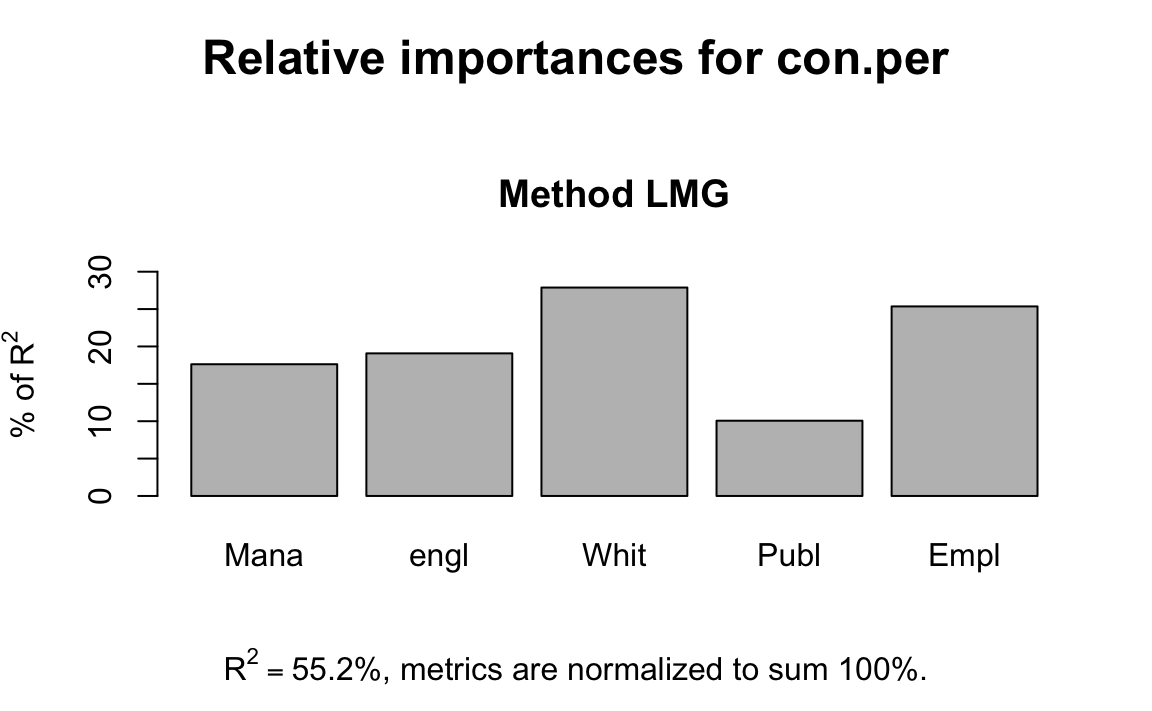
You can see that the final.model explains 55% of the variance in the percent of vote for a conservative candidate and that the White variable contributes most to the R2, followed by the Employment variable.
15.5 Multicollinearity
The regression model may experience some problems where there is strong collinearity, when the predictors are related among themselves. In these scenarios, the standard errors for the coefficients will be large and the confidence intervals will also be broader. The power of the hypothesis test for our t statistic will be lower. That is, it will be more difficult to detect a significant relationship even if there is one.
To diagnose multicollinearity a first step may be to observe the correlation between the predictors in the model. Here will we return to our merge dataset of the 2015 General Election and 2011 Census reults for parlimentary consituencies. Let’s first subset the data to only contain our outcome variable and the continuous variables in our final model.
election17aps17_sm <- subset(election17aps17, select=c(con.per, Manager,White,British,Admin,Public,Employment))Then we can obtain the correlations using the cor() function.
cor(election17aps17_sm, use="complete.obs")
#>            con.per Manager   White British   Admin Public Employment
#> con.per      1.000  0.4270  0.4007   0.171 -0.1591 -0.305     0.5040
#> Manager      0.427  1.0000  0.0763   0.189 -0.1339 -0.265     0.2968
#> White        0.401  0.0763  1.0000  -0.255  0.2079  0.202     0.3206
#> British      0.171  0.1894 -0.2552   1.000 -0.0480 -0.161     0.1408
#> Admin       -0.159 -0.1339  0.2079  -0.048  1.0000  0.795    -0.0761
#> Public      -0.305 -0.2651  0.2019  -0.161  0.7952  1.000    -0.1320
#> Employment   0.504  0.2968  0.3206   0.141 -0.0761 -0.132     1.0000
We can run the scatterplot matrix using the pairs() function:
pairs(election17aps17_sm)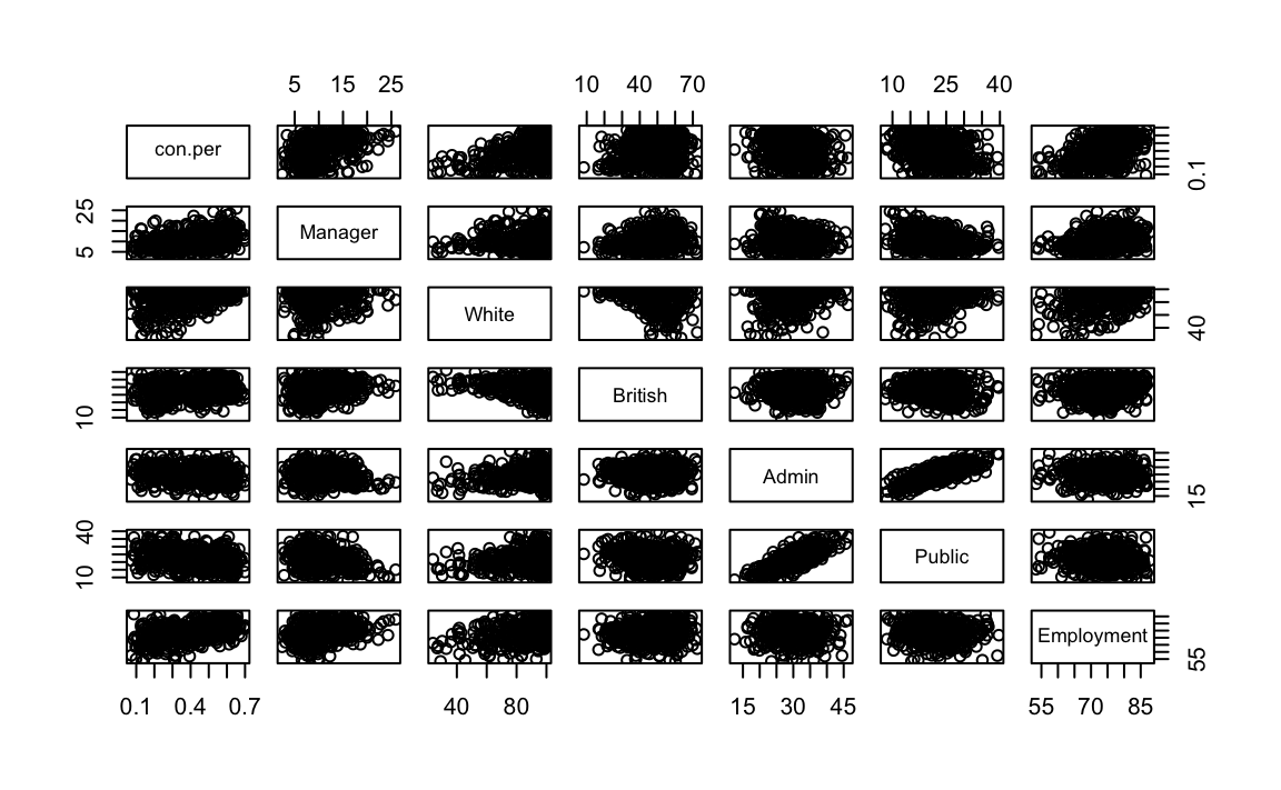
As you may have noticed the matrix is symmetrical, for every scatterplot in the upper left side there is a similar on the the bottom right side. We can modify the scatterplot matrix to display only the relationship in one direction using the option “lower.panel=NULL” or “upper.panel=NULL”.
One of the beauties of ggplot2 is that its functionality has been extended by a number of other packages. One of them is the GGally package that allows us to produce output similar to the one we just produced in one plot and extend the correlation matrix to situations in which some of your variables are not nummeric.
library(GGally)
ggpairs(election17aps17_sm)
#> plot: [1,1] [>--------------------------------------------] 2% est: 0s
#> Warning: Removed 1 rows containing non-finite values (stat_density).
#> plot: [1,2] [=>-------------------------------------------] 4% est: 3s
#> Warning in (function (data, mapping, alignPercent = 0.6, method =
#> "pearson", : Removed 3 rows containing missing values
#> plot: [1,3] [==>------------------------------------------] 6% est: 3s
#> Warning in (function (data, mapping, alignPercent = 0.6, method =
#> "pearson", : Removing 1 row that contained a missing value
#> plot: [1,4] [===>-----------------------------------------] 8% est: 4s
#> Warning in (function (data, mapping, alignPercent = 0.6, method =
#> "pearson", : Removing 1 row that contained a missing value
#> plot: [1,5] [====>----------------------------------------] 10% est: 4s
#> Warning in (function (data, mapping, alignPercent = 0.6, method =
#> "pearson", : Removing 1 row that contained a missing value
#> plot: [1,6] [=====>---------------------------------------] 12% est: 4s
#> Warning in (function (data, mapping, alignPercent = 0.6, method =
#> "pearson", : Removing 1 row that contained a missing value
#> plot: [1,7] [=====>---------------------------------------] 14% est: 3s
#> Warning in (function (data, mapping, alignPercent = 0.6, method =
#> "pearson", : Removing 1 row that contained a missing value
#> plot: [2,1] [======>--------------------------------------] 16% est: 3s
#> Warning: Removed 3 rows containing missing values (geom_point).
#> plot: [2,2] [=======>-------------------------------------] 18% est: 3s
#> Warning: Removed 2 rows containing non-finite values (stat_density).
#> plot: [2,3] [========>------------------------------------] 20% est: 3s
#> Warning in (function (data, mapping, alignPercent = 0.6, method =
#> "pearson", : Removed 2 rows containing missing values
#> plot: [2,4] [=========>-----------------------------------] 22% est: 3s
#> Warning in (function (data, mapping, alignPercent = 0.6, method =
#> "pearson", : Removed 2 rows containing missing values
#> plot: [2,5] [==========>----------------------------------] 24% est: 3s
#> Warning in (function (data, mapping, alignPercent = 0.6, method =
#> "pearson", : Removed 2 rows containing missing values
#> plot: [2,6] [===========>---------------------------------] 27% est: 3s
#> Warning in (function (data, mapping, alignPercent = 0.6, method =
#> "pearson", : Removed 2 rows containing missing values
#> plot: [2,7] [============>--------------------------------] 29% est: 3s
#> Warning in (function (data, mapping, alignPercent = 0.6, method =
#> "pearson", : Removed 2 rows containing missing values
#> plot: [3,1] [=============>-------------------------------] 31% est: 3s
#> Warning: Removed 1 rows containing missing values (geom_point).
#> plot: [3,2] [==============>------------------------------] 33% est: 3s
#> Warning: Removed 2 rows containing missing values (geom_point).
#> plot: [3,3] [===============>-----------------------------] 35% est: 3s
#> plot: [3,4] [================>----------------------------] 37% est: 3s
#> plot: [3,5] [================>----------------------------] 39% est: 3s
#> plot: [3,6] [=================>---------------------------] 41% est: 3s
#> plot: [3,7] [==================>--------------------------] 43% est: 2s
#> plot: [4,1] [===================>-------------------------] 45% est: 2s
#> Warning: Removed 1 rows containing missing values (geom_point).
#> plot: [4,2] [====================>------------------------] 47% est: 2s
#> Warning: Removed 2 rows containing missing values (geom_point).
#> plot: [4,3] [=====================>-----------------------] 49% est: 2s
#> plot: [4,4] [======================>----------------------] 51% est: 2s
#> plot: [4,5] [=======================>---------------------] 53% est: 2s
#> plot: [4,6] [========================>--------------------] 55% est: 2s
#> plot: [4,7] [=========================>-------------------] 57% est: 2s
#> plot: [5,1] [==========================>------------------] 59% est: 2s
#> Warning: Removed 1 rows containing missing values (geom_point).
#> plot: [5,2] [===========================>-----------------] 61% est: 2s
#> Warning: Removed 2 rows containing missing values (geom_point).
#> plot: [5,3] [===========================>-----------------] 63% est: 2s
#> plot: [5,4] [============================>----------------] 65% est: 1s
#> plot: [5,5] [=============================>---------------] 67% est: 1s
#> plot: [5,6] [==============================>--------------] 69% est: 1s
#> plot: [5,7] [===============================>-------------] 71% est: 1s
#> plot: [6,1] [================================>------------] 73% est: 1s
#> Warning: Removed 1 rows containing missing values (geom_point).
#> plot: [6,2] [=================================>-----------] 76% est: 1s
#> Warning: Removed 2 rows containing missing values (geom_point).
#> plot: [6,3] [==================================>----------] 78% est: 1s
#> plot: [6,4] [===================================>---------] 80% est: 1s
#> plot: [6,5] [====================================>--------] 82% est: 1s
#> plot: [6,6] [=====================================>-------] 84% est: 1s
#> plot: [6,7] [======================================>------] 86% est: 1s
#> plot: [7,1] [======================================>------] 88% est: 0s
#> Warning: Removed 1 rows containing missing values (geom_point).
#> plot: [7,2] [=======================================>-----] 90% est: 0s
#> Warning: Removed 2 rows containing missing values (geom_point).
#> plot: [7,3] [========================================>----] 92% est: 0s
#> plot: [7,4] [=========================================>---] 94% est: 0s
#> plot: [7,5] [==========================================>--] 96% est: 0s
#> plot: [7,6] [===========================================>-] 98% est: 0s
#> plot: [7,7] [=============================================]100% est: 0s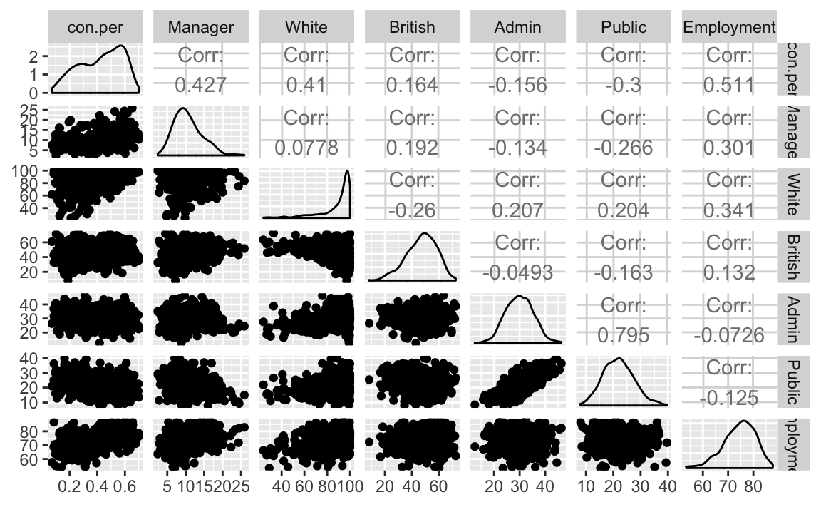
Try subsetting a data frame that contains categorical variables and try running the ggpairs function.
We can see that there are some non-trivial correlations between some of the predictors, for example, between percent working in the Public sector and percent working in Adminstration occupation (r=0.795). What can we say about the relationship between these two variables?
Correlations among pairs of variables, will only give you a first impression of the problem. What we are really concerned is what happens once you throw all the variables in the model. Not all problems with multicollinearity will be detected by the correlation matrix. The variance inflation factor can be used as a tool to diagnose multicollinearity after you have fitted your regression model. Let’s look at the VIF for our final model of the percent of votes for a conservative candidate. You might have to refit the model:
library(car)
vif(final.model)
#>    Manager    england      White     Public Employment
#>       1.17       1.23       1.25       1.27       1.26
Typically a VIF larger than 5 or 10 indicates serious problems the collinearity. Field (2012) recommends calculating the tolerance statistic, which is 1/VIF. He suggests values below 0.1 indicate a serious problem, although values below 0.2 are worthy of concern.
1/(vif(final.model))
#>    Manager    england      White     Public Employment
#>      0.851      0.811      0.800      0.789      0.794
It does not look as if we would have to worry much on the basis of these results.
When you have a multicategory factor and various dummy variables you cannot use the variance inflation factor. There is, however, a similar statistic that you can use in these contexts: the generalised variance inflation factor. R automatically invokes this statistic by recognising the multicategory factor variables in our model.
The problem with collinear inputs is that they do not add much new to the model. Non-collinearity is not an assumption of the regression model. And everything is related to everything else, to some extent at least. But if a predictor is strongly related to some other input, then we are simply adding redundant information to the model. In these situations is hard to tell apart the relative importance of the collinear predictors (if you are interested in explanation rather than prediction) and it can be difficult to separate their effects.
15.6 Acknowledgements
This exercise was adapted from R for Criminologists developed by Juanjo Medina and is licensed under a Creative Commons Attribution-Non Commercial 4.0 International License.
15.7 Additional Exercise
When running a mutiple regression model, what does it mean, statistically and conceptually, to say we are “controlling for” the effects of other variables?
Run a simple regression on
lab.per, percent of votes for a Labour candidate, using an explanatory variable of your choice and interpret the results.Add three additional explanatory variables of your choice to the model. For each variable state how it is plausibly related to lab.per. Interpret the new model (substantively and statistically). Compare your new model with your original model and report an appropiate test.
Test for multicollinearity in your model. Explain what you might do if multicollinearity was an issue.