5 Mapping in R
In this practical we will: - Load spatial data files into R - Join data to GIS spatial data files - Create a simple choropleth map - Customise choropleth maps with the tmap package
First we must set the wokring directory and load the practical data
# Remember to set the working directory as usual

# Load the data. You may need to alter the file directory
Census.Data <-read.csv("worksheet_data/camden/practical_data.csv")
5.0.1 Loading Shapefiles into R
A GIS shapefile is a file format for storing the location, shape, and attributes of geographic features. In other words, it contains the geographic information which allow it to be mapped as either points, lines or polygons. First we need to load some packages. Remember to install them first if you have not used them before. To install go to Tools > Install packages. in RStudio and enter the name of the package or use the install.packages() function. The packages are: rgdal - Bindings for the Geospatial Data Abstraction Library rgeos- Interface to Geometry Engine - Open Source
#Load Packages

library("rgdal")
library("rgeos")
Next we need to load the output area shapefile into R. Shapefiles are made up of multile different files which when combined by certain software packages can be mapped using a common projection system. We will be using output area boundaries as our data is at the output are level. Therefore, the data will be visualised as a polygon file whereby each indiviudal polygon represents the outlines of a unique output area from our study area. In this example our spatial data files can be found in the shapefiles folder of our data pack. Together this comprise: * Camden_oa11.dbf * Camden_oa11.prj * Camden_oa11.shp * Camden_oa11.shx
Before doing this please find the Camden_oa11 files from within the shapefiles folder of your census data pack you which you downloaded. Move these files to your working directory.
#Load the output area shapefile

Output.Areas <- readOGR("worksheet_data/camden", "Camden_oa11")
#> OGR data source with driver: ESRI Shapefile
#> Source: "/Users/jamestodd/Desktop/GitHub/learningR/worksheet_data/camden", layer: "Camden_oa11"
#> with 749 features
#> It has 1 fields
The inputted shapefile should contain an identical number of features as the number of observations in our Census.Data file. We can now explore the shapefile. First, we will plot it as a map to view the spatial dimensions of the shapefile mapped out. This is very simple, just enter the object name of the shapefile into the standard plot() function
#Plot the shapefile

plot(Output.Areas)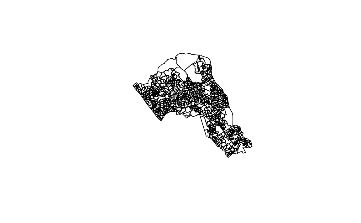
5.0.2 Joining Data
We now need to join our Census.Data to the shapefile so the census attributes can be mapped. As our census data contains the unique names of each of the output areas, this can be used a key to merge the data to our output area file (which also contains unique names of each output area). We will use the merge() function to join the data. Notice that this time the column headers for our output area names are not identical, despite the fact they contain the same data. We therefore have to use by.x and by.y so the merge function uses the correct columns to join the data.
#Join data to the shapefile
OA.Census <- merge(Output.Areas, Census.Data, by.x="OA11CD", by.y="OA")
5.0.3 Setting a coordinate system
It is also important to set a coordinate system, especially if you want to map multiple different files. The proj4string() and CRS() functions allows us to set the coordinate system of a shapefile to a predefined system of our choice. Most data from the UK is projected using the British National Grid (EPSG:27700) produced by the Ordnance Survey, this includes the standard statistical geography produced by the Office for National Statistics. We will cover map projections in more detail in the coming practicals. In this case the shapefile we originally downloaded from the CDRC Data website already has the correct projection so we don’t need to run this step for our OA.Census object. However, it is worth taking note of this step for future reference.
#Set the coordinate system to the British National Grid
proj4string(OA.Census) <- CRS("+init=epsg:27700")
#> Warning in `proj4string<-`(`*tmp*`, value = new("CRS", projargs = "+init=epsg:27700 +proj=tmerc +lat_0=49 +lon_0=-2 +k=0.9996012717 +x_0=400000 +y_0=-100000 +datum=OSGB36 +units=m +no_defs +ellps=airy +towgs84=446.448,-125.157,542.060,0.1502,0.2470,0.8421,-20.4894")): A new CRS was assigned to an object with an existing CRS:
#> +proj=tmerc +lat_0=49 +lon_0=-2 +k=0.9996012717 +x_0=400000 +y_0=-100000 +datum=OSGB36 +units=m +no_defs +ellps=airy +towgs84=446.448,-125.157,542.060,0.1502,0.2470,0.8421,-20.4894
#> without reprojecting.
#> For reprojection, use function spTransform
5.1 Mapping data in R
Whilst the plot function is pretty limited in its basic form. Several packages allow us to map data relatively easily. They also provide a number of functions to allow us to tailor and alter the graphic. ggplot2 for example allows you to map spatial data. However, probably the easiest to use are the functions within the tmap library.
#Load packages
library(tmap)
library(leaflet)
5.1.1 Creating a quick map
If you just want to create a map with a legend quickly you can use the qtm() function.
# this will prodyce a quick map of our qualification variable
qtm(OA.Census, fill = "Qualification")
5.1.2 Creating more advanced maps with tmap
Creating maps in tmap involves you binding together several functions that comprise different aspects of the graphic. For instance: polygon + polygon’s symbology + borders + layout
We enter shapefiles (or R spatial data objects) followed by a command to set their symbologies. The objects are then layered in the visualisation with the firstly entered objects at the bottom of the graphic.
5.1.2.1 Creating a simple map
Here we load in the shapefile with the tm_shape() function then add in the tm_fill() function which is where we can decide how the polygons are filled in. All we need to do in the tm_shape() function is call the shapefile. We then add (+) a separate new function (tm_fill()) to enter the parameters which will determine how the polygons are filled in the graphic. By default, we only need to include a variable name within the parameters.
You can explore all of the available functions and how they can be customised by visiting webpage for tmap, or by entering ?function into r (i.e. ?tm_fill). Below we will go through some of the basic steps of mapping with tmap.
# Creates a simple choropleth map of our qualification variable
tm_shape(OA.Census) + tm_fill("Qualification")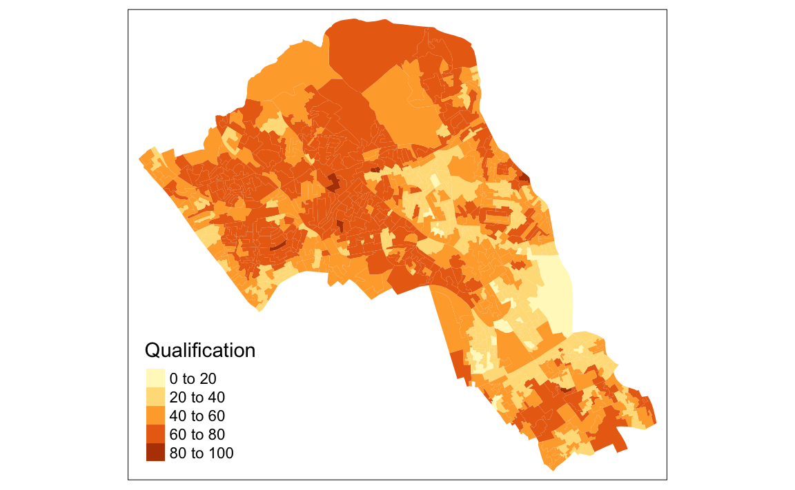
You will notice that the map is very similar to the quick map produced from using the qtm() function. However, the advantage of using the advanced functions from tmap is that they provide a wide range of customisations options. The following steps will demonstrate this.
5.1.2.2 Setting the colour palette
tmap allows you to use colour ramps either defined by the user or a set of predefined colour ramps from the RColorBrewer() function. To explore the predefined colour ramps in ColourBrewer enter the following code:
library(RColorBrewer)
display.brewer.all()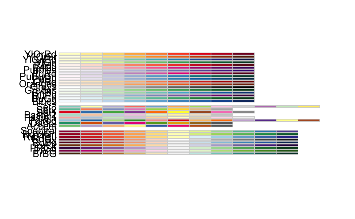
This presents a range of previously defined colour ramps. The continuous ramps at the top are all appropriate. If you enter a minus sign before the name of the ramp within the brackets (i.e. -Greens), you will invert the order of the colour ramp.
# setting a colour palette
tm_shape(OA.Census) + tm_fill("Qualification", palette = "-Greens")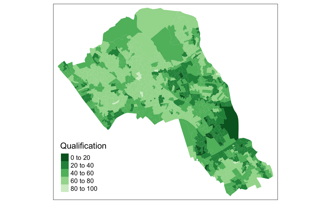
5.1.2.3 Setting the colour intervals
We have a range of different interval options in the style option. Each of them will greatly impact how your data is visualised. To do this you enter style = followed by one of the options below:
- equal - divides the range of the variable into n parts.
- pretty - chooses a number of breaks to fit a sequence of equally spaced ‘round’ values. So the keys for these intervals are always tidy and memorable.
- quantile - equal number of cases in each group
- jenks - looks for natural breaks in the data
- Cat - if the variable is categorical (i.e. not continuous data)
Try a couple of different interval styles to observe how they visualise the data differently. The example below uses the quantile interval scheme
# changing the intervals
tm_shape(OA.Census) + tm_fill("Qualification", style = "quantile", palette = "Reds")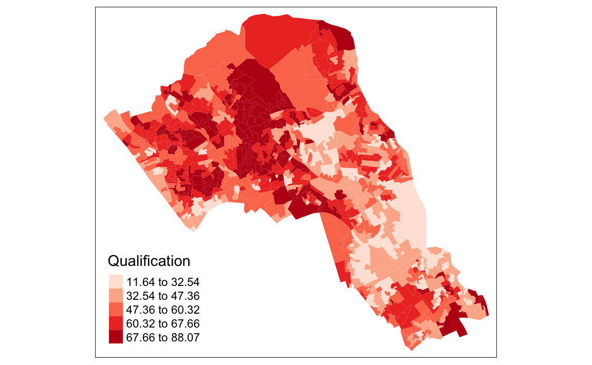
We can also change the number of intervals in the colour scheme and how the intervals are spaced. Changing the number of intervals is straight-forward, just n= n (note that the default interval setting may still round the number). Here we have 7 shades instead of the default 5.
# number of levels
tm_shape(OA.Census) + tm_fill("Qualification", style = "quantile", n = 7, palette = "Reds")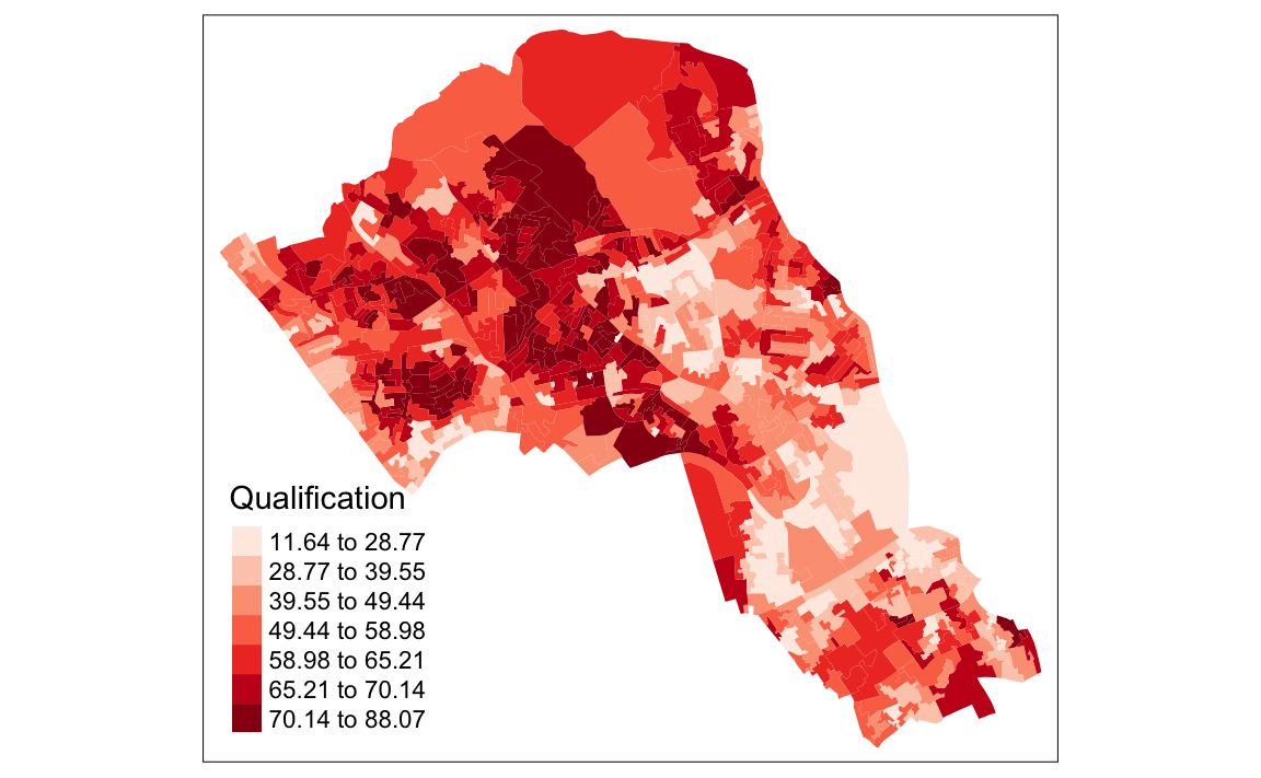
You can also create a histogram within the legend, simply add legend.hist = TRUE within tm_fill. The histogram can be quite informative of how the intervals are defined. Try running the maps with a histogram to observe how different intervals are univariately distributed across our data.
# includes a histogram in the legend
tm_shape(OA.Census) +
  tm_fill("Qualification", style = "quantile", n = 5, palette = "Reds", legend.hist = TRUE)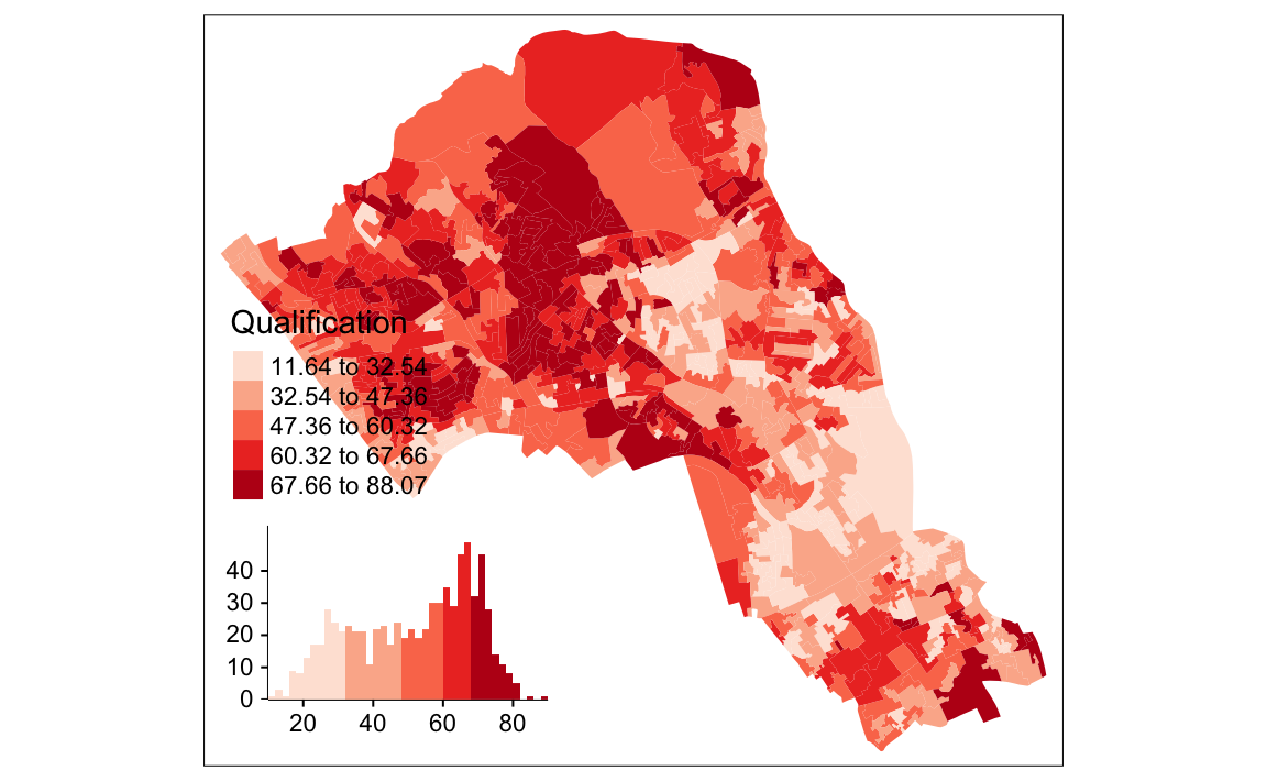
5.1.2.4 Adding borders
You can edit the borders of the shapefile with the tm_borders() function which has many arguments. alpha denotes the level of transparency on a scale from 0 to 1 where 0 is completely transparent.
# add borders
tm_shape(OA.Census) +
  tm_fill("Qualification", palette = "Reds") +
  tm_borders(alpha=.4)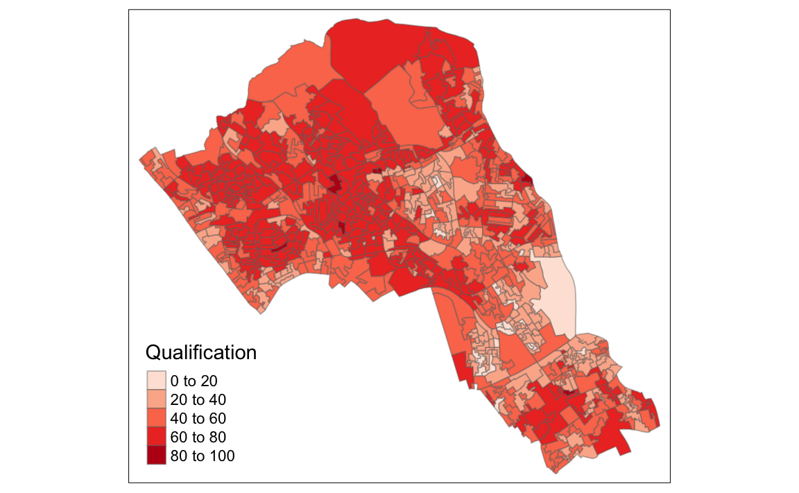
5.1.2.5 Adding a north arrow
We can also enter a north arrow with tm_compass().
# north arrow
tm_shape(OA.Census) +
  tm_fill("Qualification", palette = "Reds") +
  tm_borders(alpha=.4) +
  tm_compass()
5.1.2.6 Editing the layout of the map
It is possible to edit the layout using the tm_layout() function. In the example below we have also added in a few more commands within the tm_fill() function.
# adds in layout, gets rid of frame
tm_shape(OA.Census) +
  tm_fill("Qualification", palette = "Reds", style = "quantile",title = "% with a Qualification") +
  tm_borders(alpha=.4) +
  tm_compass() +
  tm_layout(title = "Camden, London", legend.text.size = 1.1, legend.title.size = 1.4, legend.position = c("right", "top"), frame = FALSE)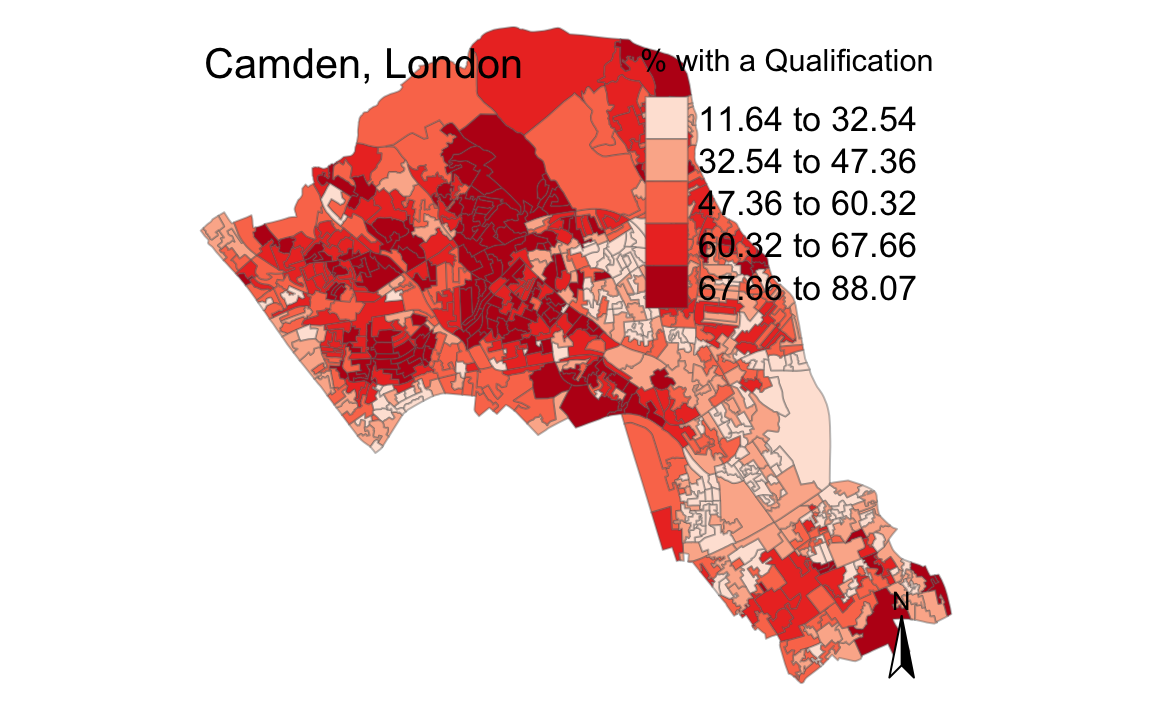
5.1.2.7 Saving the shapefile
Finally, we can save the shapefile with the Census data already attatched to by simply running the following code (remember to change the dsn to your working directory).
writeOGR(OA.Census, dsn = ".", layer = "Census_OA_Shapefile", driver="ESRI Shapefile")