7 Mapping Crime in Camden
Produce a series of maps that show the distribution of crime for Camden: - How do crimes differ between July and December? - Do particular crime types appear to cluster together? - Are they related to demographic data? (when you create the spatialpointsdataframe you need to specify a different projection code. This is done as follows: proj4string = CRS(“+init=EPSG:4326”)
First download the crime data from the data.police.uk website. In this case we are going to tick the “Metropolitan Police” box and then “July” in both the date range dropdowns. Unzip the CSV and place it in a convenient directory.
Now load in packages we need, set the working directory and load in the data. All the steps can be repeated for the December data too.
library(rgdal)
library(tmap)
#setwd("~/Dropbox/R Courses/learningR")

police_data<- read.csv("worksheet_data/camden/crime_june_19.csv")
The next step is to extract only those crimes occuring in Camden. We can us the grepl function for this. This will scan down the rows of a column we specify and extract those that contain a particular word or phrase. In our case we’re looking for Camden so the code is grepl('Camden', police_data$LSOA.name). If you run this on its own you will get a vector that contains TRUE or FALSE to indicate each row with the word. We can combine this step with the usual [ ] to select only the rows that are returned TRUE.
police_data<- police_data[grepl('Camden', police_data$LSOA.name),]Note how police_data has fewer rows in it. If you type head(police_data) you should see only Camden is present. You should also see a number of columns and recognise what some of them are for.
head(police_data)
#>                                                               Crime.ID
#> 13319
#> 13320
#> 13321
#> 13322
#> 13323
#> 13324 51a4a3926456a9157d76963407002689b3141970a11234d1d560c4429a6f0adb
#>         Month                 Reported.by                Falls.within
#> 13319 2019-07 Metropolitan Police Service Metropolitan Police Service
#> 13320 2019-07 Metropolitan Police Service Metropolitan Police Service
#> 13321 2019-07 Metropolitan Police Service Metropolitan Police Service
#> 13322 2019-07 Metropolitan Police Service Metropolitan Police Service
#> 13323 2019-07 Metropolitan Police Service Metropolitan Police Service
#> 13324 2019-07 Metropolitan Police Service Metropolitan Police Service
#>       Longitude Latitude                  Location LSOA.code   LSOA.name
#> 13319    -0.142     51.6 On or near Doynton Street E01000907 Camden 001A
#> 13320    -0.143     51.6  On or near Raydon Street E01000907 Camden 001A
#> 13321    -0.143     51.6  On or near Raydon Street E01000907 Camden 001A
#> 13322    -0.143     51.6  On or near Raydon Street E01000907 Camden 001A
#> 13323    -0.143     51.6  On or near Raydon Street E01000907 Camden 001A
#> 13324    -0.142     51.6 On or near Doynton Street E01000907 Camden 001A
#>                  Crime.type Last.outcome.category Context
#> 13319 Anti-social behaviour                            NA
#> 13320 Anti-social behaviour                            NA
#> 13321 Anti-social behaviour                            NA
#> 13322 Anti-social behaviour                            NA
#> 13323 Anti-social behaviour                            NA
#> 13324              Burglary   Under investigation      NA
Our priority here are the latitude and longitude columns in order that we can create a dot map. It is worth noticing, however, that some locations have had more than one crime occur. If we did a plot of these they would appear on top of one another so its better to aggregate these to create a data frame that has the number of crimes of each type by location. To do this we need to use the aggregate() function on the Longitude, Latitude, LSOA.code (this will be useful later), and Crime.type columns.
#By unsing FUN=length we are asking that the aggregate function counts the number of times a crime.ID appears at a location.
crime_count<- aggregate(police_data$Crime.ID, by=list(police_data$Longitude, police_data$Latitude,police_data$LSOA.code,police_data$Crime.type), FUN=length)

#We need to rename our columns (note these are abbreviated from the originals)
names(crime_count)<- c("Long","Lat","LSOA","Crime","Count")
Now we are ready to convert this to spatial data object in R by specifying that the Long/Lat columns (columns 1 & 2) contain this information. Note that we specify EPSG: 4326 as our projection system.
crime_count_sp<- SpatialPointsDataFrame(crime_count[,1:2], crime_count, proj4string = CRS("+init=epsg:4326"))We’re now ready to produce a simple map using tmap. To add the additional layers such as the LSOA boundaries and demographic data revisit the “Mapping Point Data in R” worksheet. In the code below both the size of the bubble represents the count of the crimes and its colour is determined by type of crime that occured.
  tm_shape(crime_count_sp) + tm_bubbles(size = "Count", col = "Crime", legend.size.show = FALSE) +
  tm_layout(legend.text.size = 1.1, legend.title.size = 1.4, frame = FALSE)
#> Some legend labels were too wide. These labels have been resized to 0.74, 0.57, 0.66, 0.72, 0.53. Increase legend.width (argument of tm_layout) to make the legend wider and therefore the labels larger.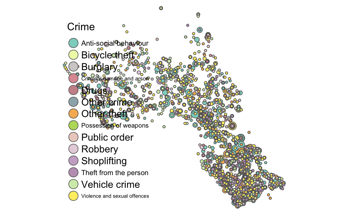
You can adjust some of the colour parameters etc to make this map look a little clearer. However, you will notice that there is a lot of overplotting as different crime types in the same location are plotted one on top of another. tmap has a clever function called tm_facets that will create one map for each crime type for us.
  tm_shape(crime_count_sp) + tm_bubbles(size = "Count", legend.size.show = FALSE) +
  tm_layout(legend.text.size = 1.1, legend.title.size = 1.4, frame = FALSE)+tm_facets(by="Crime")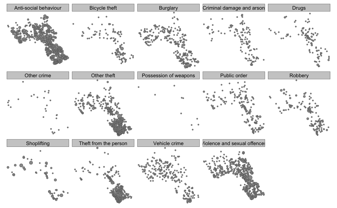
We can then make this a bit clearer with some transparency on the circles using the alpha= parameter.
  tm_shape(crime_count_sp) + tm_bubbles(size = "Count", legend.size.show = FALSE, alpha=0.5) +
  tm_layout(legend.text.size = 1.1, legend.title.size = 1.4, frame = FALSE)+tm_facets(by="Crime")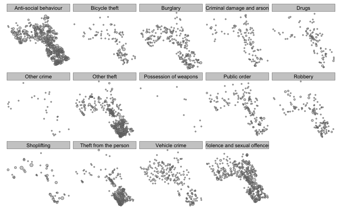
There’s a lot you can do to build up these plots further - so play around with the different options.
7.0.1 Aggregating to Polygon Data
Another way to investigate crimes in Camden would be to count the number of crimes in each LSOA and map it.
At the moment we have our data organised with the crime types as separate rows. So each LSOA will have multiple rows - one per count of crime type. We can’t join these rows to our spatial data object, we need one row per LSOA to match it. Therefore we should create a table with columns for each crime type and a single row per LSOA. In technical terms we need to go from a long format to a wide format for the data. For this we go back to the police_data object (before it was converted to a spatial format) and we use the spread function to create the format we need. You first need to install the tidyr package and then load it.
library(`tidyr`)

#First aggregate the data to each LSOA (rather than the specific latitude and longitude as we did before)

crime_LSOA<- aggregate(police_data$Crime.ID, by=list(police_data$LSOA.code,police_data$Crime.type), FUN=length)

#We need to rename our columns (note these are abbreviated from the originals)
names(crime_LSOA)<- c("LSOA","Crime","Count")

# The arguments to spread():
# - data: Data object
# - key: Name of column containing the new column names
# - value: Name of column containing values

crime_LSOA<- spread(crime_LSOA,Crime, Count)
If you look at the data frame we’ve just created it is is now possible to see we have columns for each crime type and their counts (NAs mean there was no reported crime). Now we can join to our spatial object. For this we need the camden_lsoa11.shp file. Note it is lsoa11 NOT oa11 so you may need to revisit the original folder downloaded in last weeks practical.
LSOA<- readOGR("worksheet_data/camden","Camden_lsoa11")
#> OGR data source with driver: ESRI Shapefile
#> Source: "/Users/jamestodd/Desktop/GitHub/learningR/worksheet_data/camden", layer: "Camden_lsoa11"
#> with 133 features
#> It has 1 fields
If we look at the head() of the LSOA object we can see what field in its data frame we can use to join the crime object to.
head(LSOA@data)
#>    LSOA11CD
#> 0 E01000842
#> 1 E01000843
#> 2 E01000844
#> 3 E01000845
#> 4 E01000846
#> 5 E01000847
In this case there is only one column LSOA11CD, which as -luck would have it- is what we need!
LSOA_crime_sp<- merge(LSOA, crime_LSOA, by.x="LSOA11CD", by.y="LSOA")
#Check the head of the new file to see if it worked.
head(LSOA_crime_sp@data)
#> LSOA11CD Anti-social behaviour Bicycle theft Burglary
#> 1 E01000842 1 1 NA
#> 2 E01000843 8 NA 1
#> 3 E01000844 1 2 NA
#> 4 E01000845 16 1 3
#> 5 E01000846 1 1 NA
#> 6 E01000847 5 NA 1
#> Criminal damage and arson Drugs Other crime Other theft
#> 1 NA NA NA 1
#> 2 1 NA 1 2
#> 3 1 NA NA 2
#> 4 NA 1 NA NA
#> 5 NA NA NA NA
#> 6 NA NA NA 3
#> Possession of weapons Public order Robbery Shoplifting
#> 1 NA NA NA NA
#> 2 NA 1 NA NA
#> 3 NA 1 1 NA
#> 4 NA NA 2 NA
#> 5 NA 1 1 NA
#> 6 NA NA 1 NA
#> Theft from the person Vehicle crime Violence and sexual offences
#> 1 NA 2 3
#> 2 NA NA 1
#> 3 NA 3 1
#> 4 NA 3 5
#> 5 2 3 1
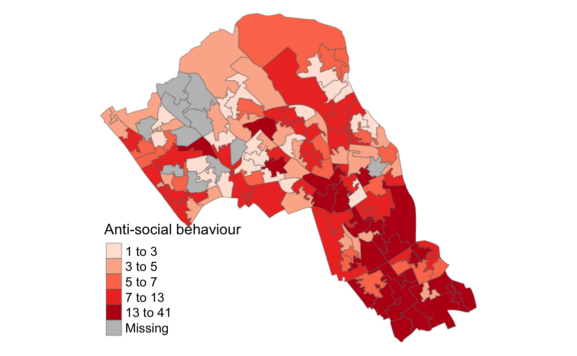
#> 6 NA 2 7Phew! Almost there! We’ve now got our spatial object with the counts per crime that are ready for mapping. Here we map the counts of Anti-social behaviour in the borough.
tm_shape(LSOA_crime_sp) +
  tm_fill("Anti-social behaviour", palette = "Reds", style = "quantile", title = "Anti-social behaviour") +
  tm_borders(alpha=.4) + tm_layout(legend.text.size = 0.8, legend.title.size = 1.1, frame = FALSE)