11 Interpolating Point Data
In this practical we will: - Create thiessen polygons - Run an inverse distance weighting to interpolate point data - Clip a spatial data using the crop (for polygons) and mask (for rasters) functions
First we must set the working directory and load the practical data.
# Remember to set the working directory as usual

# Load the data. You may need to alter the file directory
Census.Data <-read.csv("worksheet_data/camden/practical_data.csv")
We will also need the load the spatial data files from the previous practicals.
# load the spatial libraries
library("sp")
library("rgdal")
library("rgeos")
library("tmap")

# Load the output area shapefiles
Output.Areas <- readOGR("worksheet_data/camden", "Camden_oa11")
#> OGR data source with driver: ESRI Shapefile
#> Source: "/Users/jamestodd/Desktop/GitHub/learningR/worksheet_data/camden", layer: "Camden_oa11"
#> with 749 features
#> It has 1 fields
# join our census data to the shapefile
OA.Census <- merge(Output.Areas, Census.Data, by.x="OA11CD", by.y="OA")

# load the houses point files
House.Points <- readOGR("worksheet_data/camden", "Camden_house_sales")
#> OGR data source with driver: ESRI Shapefile
#> Source: "/Users/jamestodd/Desktop/GitHub/learningR/worksheet_data/camden", layer: "Camden_house_sales"
#> with 2547 features
#> It has 4 fields
#> Integer64 fields read as strings:  UID Price oseast1m osnrth1m
11.1 Why interpolate data
There are many reasons why we may wish to interpolate point data across a map. It could be because we are trying to predict a variable across space, including in areas where there are little to no data. As exemplified by house price heat maps on major property websites (see below).
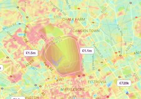
A estimating the spatial distribution of house prices across Camden and the surrounding area. Source: Zoopla.co.uk
We might also want to smooth the data across space so that we cannot interpret the results of individuals, but still identify the general trends from the data. This is particularly useful when the data corresponds to individual persons and disclosing their locations is unethical.
11.1.1 Thiessen polygons
The first step we can take to interpolate the data across space is to create Thiessen polygons. Thiessen polygons are formed to assign boundaries of the areas closest to each unique point. Therefore, for every point in a dataset, it has a corresponding Thiessen polygon. This is demonstrated in the diagram below.
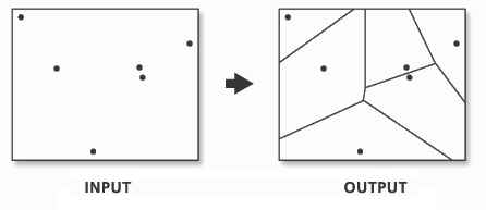
A demonstration of Thiessen polygon generation from point data. Source: resources.esri.com
So in this exercise, we will create Thiessen polygons for our house data, then use the polygons to map the house prices of their corresponding house point. The spatstat package provides the functionality to produce Thiessen polygons via its dirichelet tesselllation of spatial point patterns function (dirichlet()). We also need to first convert the data to a ppp (spatial point pattern) object class. The maptools package will enable the as.ppp() function.
library(spatstat)
library(maptools)  # Needed for conversion from SPDF to ppp

# Create a tessellated surface
dat.pp <- as(dirichlet(as.ppp(House.Points)), "SpatialPolygons")
dat.pp <- as(dat.pp,"SpatialPolygons")

# Sets the projection to British National Grid
proj4string(dat.pp) <- CRS("+init=EPSG:27700")
proj4string(House.Points) <- CRS("+init=EPSG:27700")

# Assign to each polygon the data from House.Points
int.Z <- over(dat.pp,House.Points, fn=mean)

# Create a SpatialPolygonsDataFrame
thiessen <- SpatialPolygonsDataFrame(dat.pp, int.Z)


# maps the thiessen polygons and House.Points
tm_shape(OA.Census) + tm_fill(alpha=.3, col = "grey") +
tm_shape(thiessen) +  tm_borders(alpha=.5, col = "black") +
tm_shape(House.Points) + tm_dots(col = "blue", scale = 0.5)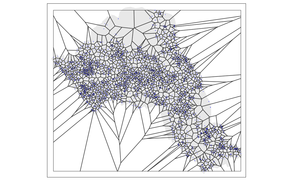
From the map you can interpret the nearest neighbourhoods for each point. We can also clip the Thiessen polygon by the OA.Census shapefile so it only represents the borough of Camden. We will do this using the crop() function from the raster package.
library(raster)
# crops the polygon by our output area shapefile
thiessen.crop <-crop(thiessen, OA.Census)

# maps cropped thiessen polygons and House.Points
tm_shape(OA.Census) + tm_fill(alpha=.3, col = "grey") +
tm_shape(thiessen.crop) +  tm_borders(alpha=.5, col = "black") +
tm_shape(House.Points) + tm_dots(col = "blue", scale = 0.5)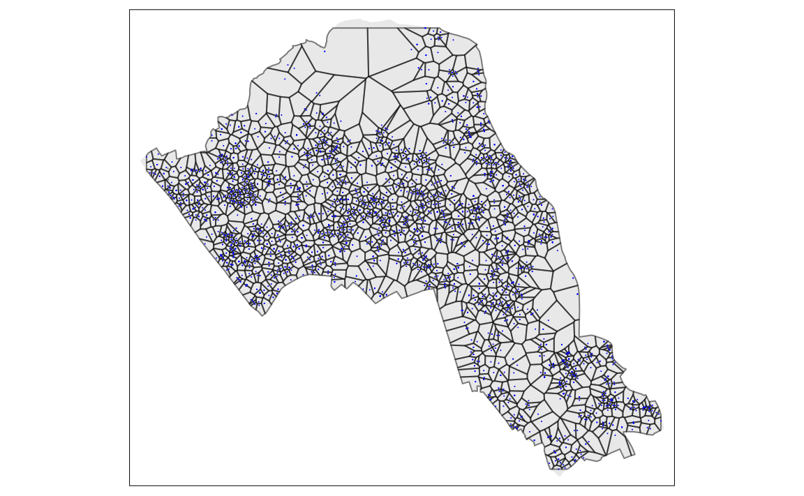
We can now map our point data using the newly formed polygons.
# maps house prices across thiessen polygons
tm_shape(thiessen.crop) + tm_fill(col = "Price", style = "quantile", palette = "Reds", title = "Price Paid (?)") + tm_borders(alpha=.3, col = "black") +
tm_shape(House.Points) + tm_dots(col = "black", scale = 0.5) +
tm_layout(legend.position = c("left", "bottom"),  legend.text.size = 1.05, legend.title.size = 1.2, frame = FALSE)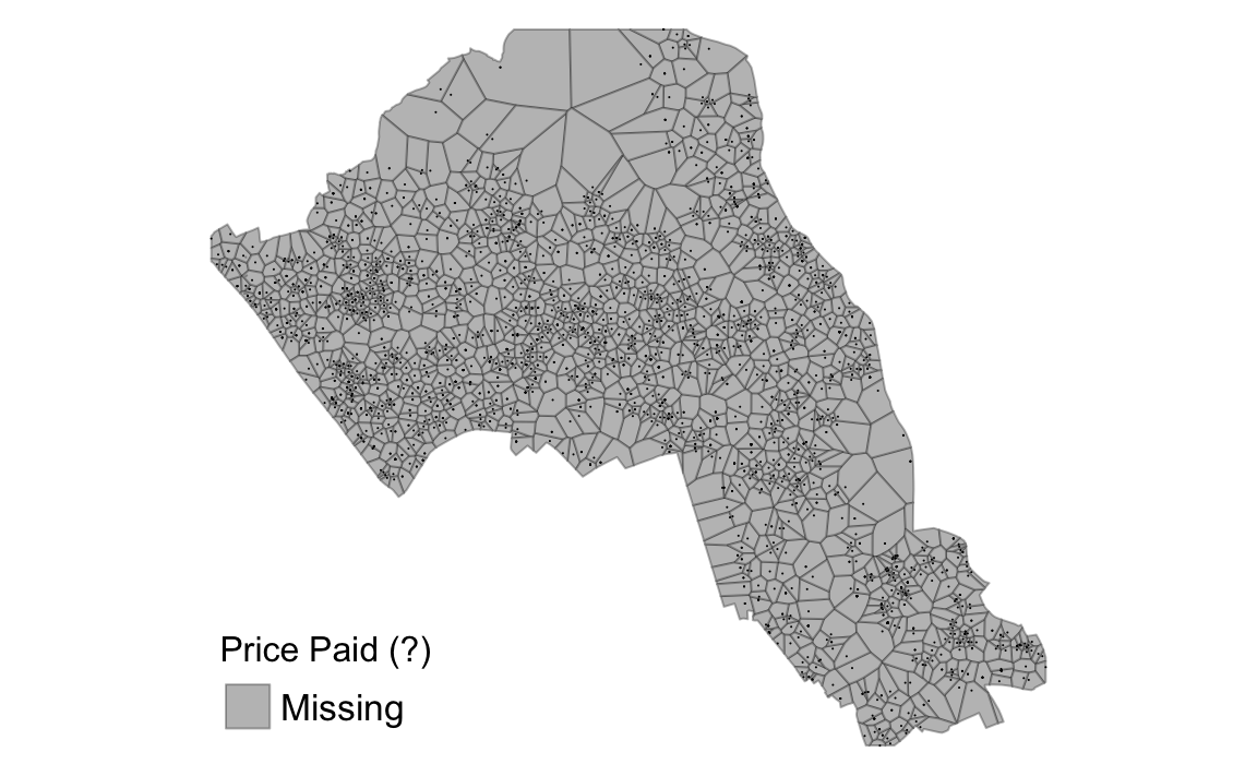
11.1.2 Inverse Distance Weighting (IDW)
An IDW is a means of converting point data of numerical values into a continuous surface to visualise how the data may be distributed across space, including spaces where no data are present. The technique interpolates point data by using a weighted average of a variable from nearby points to predict the value of that variable for each location. The weighting of the points is determined by their inverse distances drawing on Tobler’s first law of geography that “everything is related to everything else, but near things are more related than distant thing”. The output is most commonly represented as a raster surface.
To run an IDW we will need to run the code below which will interpolate the price variable of our House.Points object.
library(gstat)
library(xts)

# define sample grid based on the extent of the House.Points file
grid <-spsample(House.Points, type = 'regular', n = 10000)

# runs the idw for the Price variable of House.Points
idw <- idw(House.Points$Price ~ 1, House.Points, newdata= grid)
#> [inverse distance weighted interpolation]
The IDW is outputted to a data type, but more needs to be done before it can be visualised. We will first transform the data into a data frame data type. We can then rename the column headers.
idw.output = as.data.frame(idw)
names(idw.output)[1:3] <- c("long", "lat", "prediction")
Next we need to convert this data into a raster, the raster can then be plotted on a map along with our other spatial data.
library(raster) # you will need to load this package if you have not done so already

# create spatial points data frame
spg <- idw.output
coordinates(spg) <- ~ long + lat

# coerce to SpatialPixelsDataFrame
gridded(spg) <- TRUE
# coerce to raster
raster_idw <- raster(spg)

# sets projection to British National Grid
projection(raster_idw) <- CRS("+init=EPSG:27700")

# we can quickly plot the raster to check its okay
plot(raster_idw)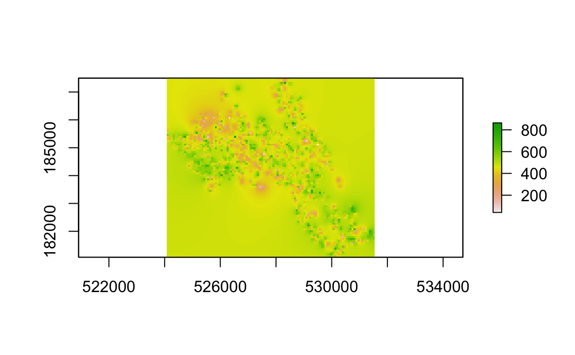
Its even possible to make a 3D plot, by very simply using the persp() function. Simply enter persp(raster_idw) into R.
persp(raster_idw)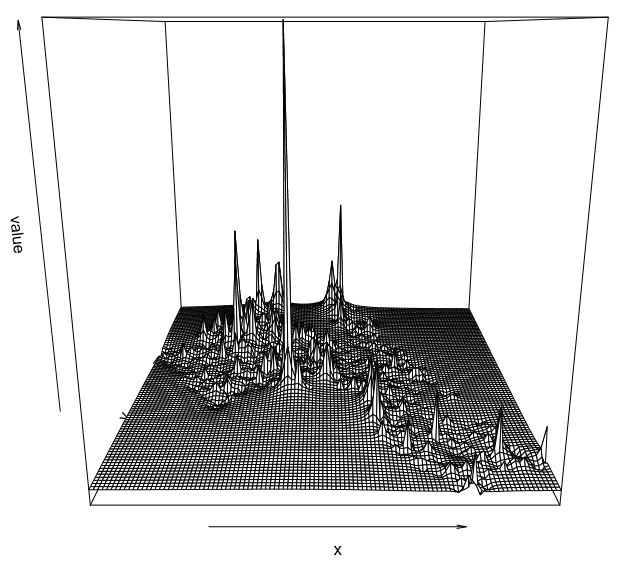
We can also create a 3D interactive chart using the rgl package and its persp3d() function.
# this package lets us create interactive 3d visualisations
library(rgl)

# we need to first convert the raster to a matrix object type
idw2 <- as.matrix(raster_idw)

persp3d(idw2, col = "red")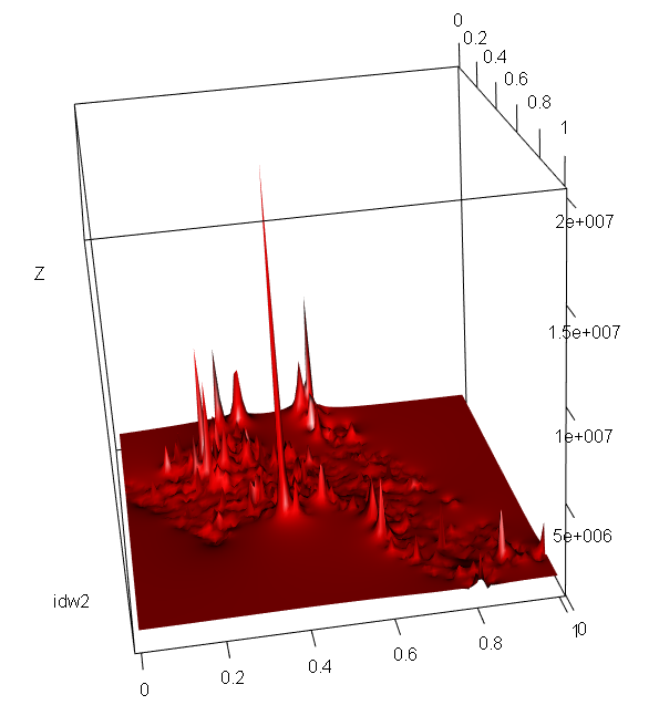
Now we are ready to plot the raster. As with our previous practicals, we will use the functionality of the tmap package, using the tm_raster() function. The instructions below will create a smoothed surface. In the example we have created 100 colour breaks and turned the legend off, this will create a smoothed colour effect. You can experiment by changing the breaks (n) to 7 and turning the legend back on (legend.show) to make the predicted values easier to interpret.
library(tmap)
tm_shape(raster_idw) + tm_raster("prediction", style = "quantile", n = 100, palette = "Reds", legend.show = FALSE) 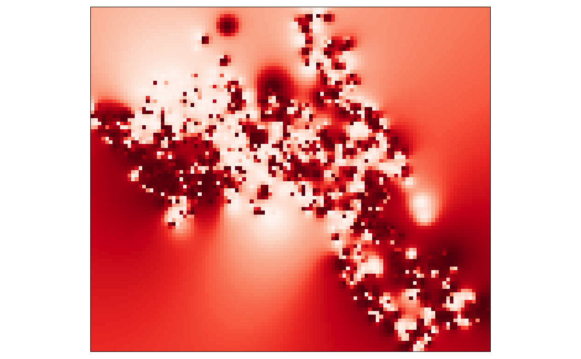
It is also possible to overlay the output area boundaries to provide some orientation. This requires us to load the OA.Census shapefie with tm_shape().
tm_shape(raster_idw) + tm_raster("prediction", style = "quantile", n = 100, palette = "Reds", legend.show = FALSE) +
tm_shape(OA.Census) + tm_borders(alpha=.5)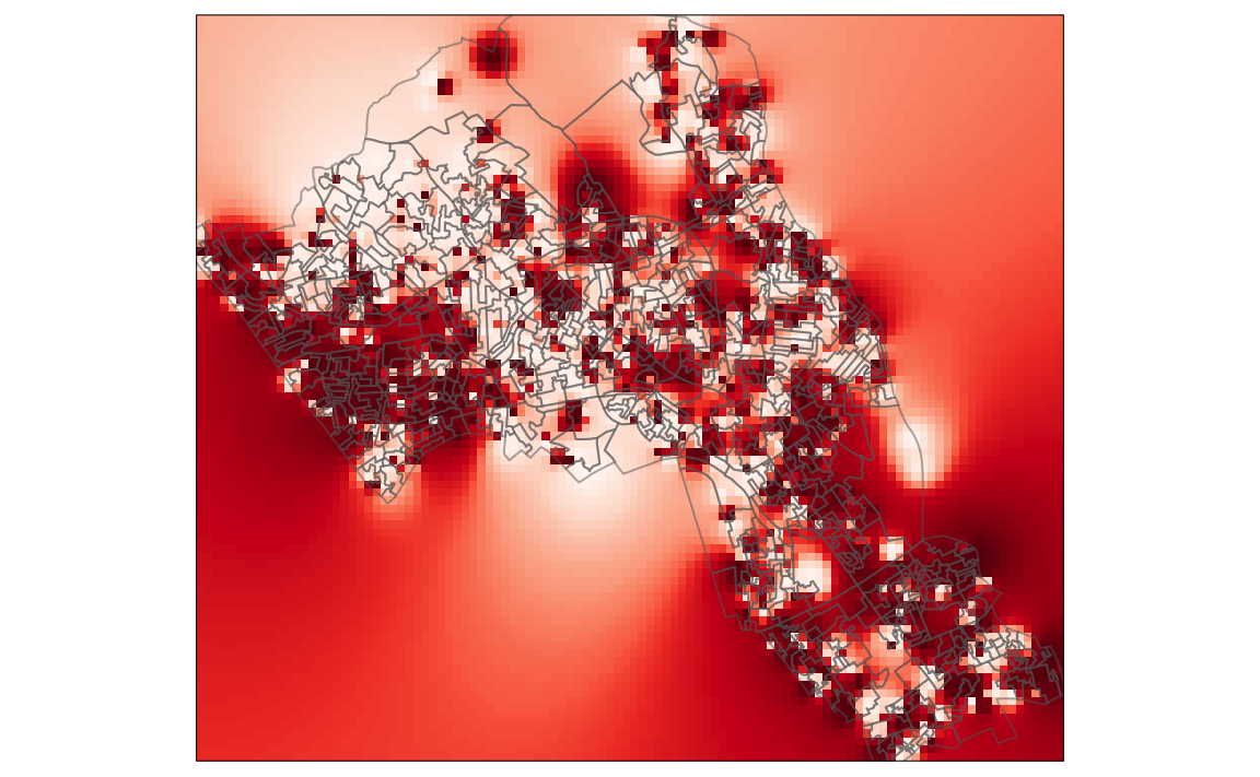
We can also overlay the original house price data as this provides a good demonstration of how the IDW is distributed. In the example we have also edited the layout. Notice that we have made the legend background white (legend.bg.color) and also made it semi-transparent (legend.bg.alpha).
tm_shape(raster_idw) + tm_raster("prediction", style = "quantile", n = 100, palette = "Reds",legend.show = FALSE) +
tm_shape(OA.Census) + tm_borders(alpha=.5) +
tm_shape(House.Points) + tm_bubbles(size = "Price", col = "Price", palette = "Blues", style = "quantile", legend.size.show = FALSE, title.col = "Price Paid (?)") +
tm_layout(legend.position = c("left", "bottom"),  legend.text.size = 1.1, legend.title.size = 1.4, frame = FALSE, legend.bg.color = "white", legend.bg.alpha = 0.5)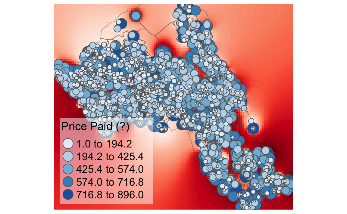
11.1.3 Masking a raster
Masking is a GIS process of when a raster is clipped using the outline of another shapefile. In this case we will clip the raster so it only shows areas within the borough of Camden. The mask function is enabled by the raster package of which we have already loaded.
# masks our raster by our output areas polygon file
masked_idw <- raster::mask(raster_idw, OA.Census)

# plots the masked raster
tm_shape(masked_idw) + tm_raster("prediction", style = "quantile", n = 100, legend.show = FALSE) +
tm_shape(House.Points) + tm_bubbles(size = "Price", col = "Price", palette = "Blues", style = "quantile", legend.size.show = FALSE, title.col = "Price Paid (?)") +
tm_layout(legend.position = c("left", "bottom"),  legend.text.size = 1.1, legend.title.size = 1.4, frame = FALSE)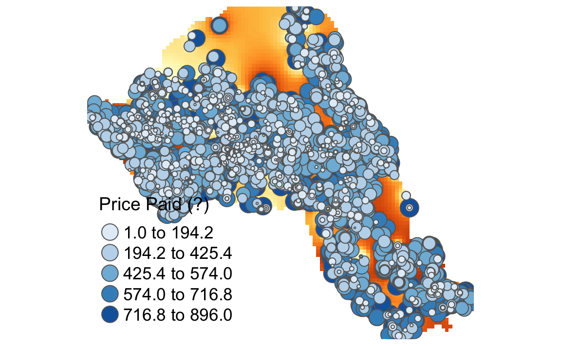
11.1.4 Geostatistical interpolation
An IDW is not the only means of interpolating point data across space. A range of geostatistical techniques have also been devised. One of the most commonly used is kriging. Whilst an IDW is created by looking at just known values and their linear distances, a kriging also considers spatial autocorrelation. The approach is therefore more appropriate is there is a known spatial or directional bias in the data. Kriging is a statistical model which uses variograms to calculate the autocorrelation between points and distance. Like an IDW the the values across space are estimated from weighted averages formed by the nearest points and considers the influence of distance. However, the approach is also geostatistical given that the weights are also determined by a semivariogram.
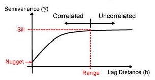
A Semivariogram
There are various different ways of running a kriging, some are quite complex given that the method requires an experimental variogram of the data in order to run.
However, the automap package provides the simplest means of doing this.
library(automap)
## Warning: package 'automap' was built under R version 3.3.1
# this is the same grid as before
grid <-spsample(House.Points, type = 'regular', n = 10000)

# runs the kriging
kriging_result = autoKrige(log(Price)~1, House.Points, grid)

plot(kriging_result)