18 Missing data
18.1 Item non-response
Item non-response is a situation in data analysis where partial data are available for a respondent. This is often referred to as missing data. It is different from unit non-response that we saw last week that can be adjusted for by using sample weights. Missing data or item non-response is often ignored and many data analyst report what is referred to as a complete case analysis. There are situations when this is appropiate and others when it is not. This decision can be made on the basis of the missing data, or to put another way, to understand why they are missing. There are broadly three missing data mechanisms that we can describe:
- Missing Completely at Random (MCAR)
If data are Missing Completely at Random (MCAR), then consistent results would be obtained using complete case analysis as would be obtained had there been no missing data, although there would be some loss of information and a smaller sample size. An example of a MCAR mechanism is where a survey question is only asked of a simple random sample of respondents. This could be intentional to test a new question in an existing survey. For example, in the English Longitudinal Study of Ageing the sample was randomly split in half in 2004 with one half answering a question on self-rated health with different response categories to the other. This was to test two versions of a self-rated health question that were asked differently in the Health Survey for England compared with the Census of Population.
- Missing at random (MAR)
Most missingness is not completely at random. For example, the different non-response rates of income across age and social class groups suggest that these data are not completely missing at random.
Missing at random assumes that the probability of missingness depends only on other variables that are available. For example, if age and social class are recorded for all people in the survey, then income can be declared as missing at random if the probability of missing on this item depends only on these known variables. This is often tested using logistic regression - which will be introduced in Term 2 - where the outcome variable equals 1 for missing values and 0 for observed values, or vice versa.
When an outcome variable is deemed to be missing at random, it is acceptable to exclude the missing respondents, providing the regression model controls for all the variables known to affect the probability of missingness to avoid bias.
- Missing not at random (MNAR)
When neither MCAR nor MAR hold, we say the data are Missing Not At Random (MNAR). This refers to a situation where even accounting for all the available observed information, the reason for observations being missing still depends on the unseen observations themselves. For example, respondents with low income are less likely to report income. Unfortunately, we cannot tell from the data at hand whether the missing observations are MCAR, MAR or MNAR (although we can distinguish between MCAR and MAR). And to complicate matters further, most imputation methods used by statisticians work under the assumption that data are missing at random. All is not lost, however. Using imputation, especially multiple imputation to address non-response is not likely to remove bias completely, but it is reasonable to expect bias to be reduced when compared with an analysis that simply drops the missing observations (i.e. complete case analysis).
18.2 Missing data in R
In UK Data Service datasets (e.g. HSE), the data providers usually code the missing values using negative values, indicating the reason for the missingness (e.g. not applicable, refused, don’t know). While this is informative for the data analyst, it requires more careful selection of variables that should and should not be deemed as missing. We will simply recode all these values to NA, the value that denotes a true missing value in R. Let’s do this for mental wellbeing (wemwbs), equivalised income (eqvinc) and body mass index (bmival) variables using our hse_and_shes12 dataset.
hse_and_shes12$wemwbs[hse_and_shes12$wemwbs<0] <- NA
hse_and_shes12$eqvinc[hse_and_shes12$eqvinc<0] <- NA
hse_and_shes12$bmival[hse_and_shes12$bmival<0] <- NA
The mean values on these variables should be higher now that we have removed the missing values that were originaly coded as negative values. When using the lm function, R will automatically exclude the missing values NA and conduct a complete case analysis. Other base package functions, such as, mean will require you to state that there are missing values.
mean(hse_and_shes12$wemwbs)
#> [1] NA
mean(hse_and_shes12$wemwbs, na.rm=TRUE)
#> [1] 51.3
18.3 Mean imputation
Rather than removing missing values from our analysis, another approach is to fill or “impute” missing values. A selection of imputation approaches can be applied, ranging from relatively simple to rather complex. These methods retain the full sample size, which can be advantageous for bias and precision, but they can result in different kinds of bias. Mean imputation is perhaps the most basic method to replace missing values with the mean of an observed value. This methods can distort the distribution for the variable leading to underestimates of the standard deviation. Moreover, mean imputation distorts relationships between variables by “pulling” estimates of the correlation toward zero. There are functions designed to do this in R, but let’s start by using the ifelse function of the base package. The code tests each case of eqvinc; if it is NA, it is replace with its mean and is saved as a new variable eqvinc_meanimp.
hse_and_shes12 = transform(hse_and_shes12, eqvinc_meanimp = ifelse(is.na(eqvinc), mean(eqvinc, na.rm=TRUE), eqvinc))Check the mean value of your new variable eqvinc_meanimp and its distribution using the hist function
mean(hse_and_shes12$eqvinc_meanimp)
#> [1] 33632
hist(hse_and_shes12$eqvinc_meanimp)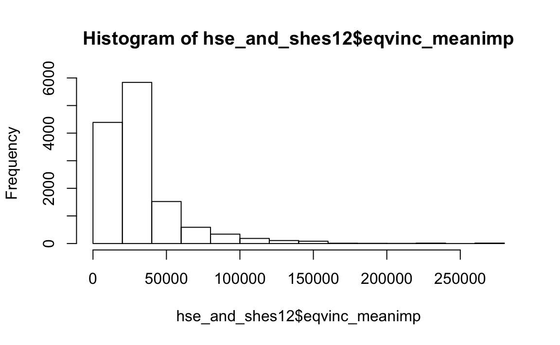
How does it compare to the original variable?
A slightly more complicated form of imputation is regression imputation where missing values are replaced with predicted score from a regression equation. This method will not distort the covariance, but will lead to overestimation. It is therefore unlikely to reduce the bias in missing data anymore than mean imputation.
18.4 Hot-deck imputation
A different way to impute is through matching: for each respondent (called the recipient) with a missing y, find a respondent (donor) with similar values of X in the observed data and take its y value. This approach is called “hot-deck” imputation. Hot-deck imputation is widely used, however the theory that supports it is not nearly as extensive as other imputation methods, such as multiple imputation. In some versions of hot-deck imputation the donor is selected randomly, in others a single donor is identified, usually the “nearest neighbour” based on some metric. A variant of hot-deck imputation has been used to produce finalised outputs for national censuses and surveys, including the 2011 Census for England and Wales.
Here we will work through an example of a sequential hot-deck imputation which imputes the missing values in any variable by replicating the most recently observed value in that variable. We will use the HotDeckImputation package. The impute.SEQ_HD function requires our data to be a matrix, which we can create using the following code:
hse_and_shes12.matrix<-data.matrix(hse_and_shes12, rownames.force = NA)Now run the impute.SEQ_HD function.
library(HotDeckImputation)
hse_and_shes12.hotdeck<-cbind(impute.SEQ_HD(DATA=hse_and_shes12.matrix,initialvalues=0, navalues=NA, modifyinplace = FALSE),hse_and_shes12.matrix)
Take a look at the dataset you have just created and you will see that each missing value has been replaced by the previous non-missing value when a missing value was specified as NA. The HotDeckImputation package allows more complicated forms of hot-deck imputation as well as a simple mean imputation method that will allow you to impute mean values across your entire dataset.
hse_and_shes12.matrix<-impute.mean(DATA=hse_and_shes12.matrix)18.5 Multiple imputation
The imputation methods we have looked at so far replace missing values with one random (or non-random) value. An alternative approach is to impute several values that reflect the uncertainty in our imputations. Multiple imputation does this by creating several imputed values for each missing value. It is common to start with five imputations, but analyst often impute many more in their final analysis. Each value is predicted with a slightly different model and therefore produces a different value that reflects sampling variability, thus produces variability that is more accurate. You should include all variables you plan to use in your analysis (e.g. regression model) in the imputation, not only those that contain missing values. A preferable approach is to also include variables in your data that are related to the missingness that might not be part of your analysis. This will ensure you are more certain about the missing at random assumption that multiple imputation relies upon.
The main disadvantage of multiple imputation is that it adds an increased level of complexity to your analysis that you have to understand and explain to your audience. In R, there are a range of competing packages that will perform multiple imputation, including mice, Amelia, mi and mitools. If you plan to take account of complex survey design, mitools is perhaps the preferred option. We will use the aregImpute function from the Hmisc package because it is easier and faster to use than most of the others. It uses predictive mean matching to impute missing values, we need not worry what this means at this stage.
Let’s run an imputation using the income, mental wellbeing, age, sex and body mass index variables to impute five datasets. The function argImpute will automatically identify the variable type and treat them accordingly.
library(Hmisc)
hse_and_shes12.mi <- aregImpute(~ eqvinc + wemwbs + age + Sex + bmival, data = hse_and_shes12, n.impute = 5)
#> Iteration 1
Iteration 2
Iteration 3
Iteration 4
Iteration 5
Iteration 6
Iteration 7
Iteration 8
You will probably get an error message. How can you correct this? You will first need to remove the redundant levels in your Sex variable. Rerun the imputation once you have figured it out.
Then you can call on your imputation:
hse_and_shes12.mi
#>
#> Multiple Imputation using Bootstrap and PMM
#>
#> aregImpute(formula = ~eqvinc + wemwbs + age + Sex + bmival, data = hse_and_shes12,
#>     n.impute = 5)
#>
#> n: 13106     p: 5    Imputations: 5      nk: 3
#>
#> Number of NAs:
#> eqvinc wemwbs    age    Sex bmival
#>   2368   3858      0      0   2152
#>
#>        type d.f.
#> eqvinc    s    2
#> wemwbs    s    2
#> age       s    2
#> Sex       c    1
#> bmival    s    1
#>
#> Transformation of Target Variables Forced to be Linear
#>
#> R-squares for Predicting Non-Missing Values for Each Variable
#> Using Last Imputations of Predictors
#> eqvinc wemwbs bmival
#>  0.051  0.055  0.061
You’ll see from the output that there were no missing values for age or sex, but thousands for income, mental wellbeing and BMI. We can ignore the rest of the output for now.
You can also call upon the imputed values for summary statistics. We don’t have to specify na.rm=TRUE anymore. Why?
mean(hse_and_shes12.mi$imputed$eqvinc)
#> [1] 31535
sd(hse_and_shes12.mi$imputed$eqvinc)
#> [1] 28437
How does this compare to the complete case mean and the sequential hot-deck imputation mean and standard deviation for income? And why are your values different from mine, the person sat next to you and everyone else in the room? Run the imputation again and see what happens to the value of your multiple imputed mean of income. Remember the practical in POLS0008 when we created a random variable and we wanted to ensure everyone produced the same value we used set.seed(). Try setting a seed (e.g. set.seed(22)) before you run your imputation to see if you can reproduce the same result twice.
The Hmisc package also has a function to impute mean values:
hse_and_shes12$eqvinc_meanimp2 <- with(hse_and_shes12, impute(eqvinc, mean))You can replace the mean option with random, min, max, median to impute missing values. This is more useful for creating variables that are a summary of categories across your data (e.g. difference between age of partners in a household).
The required function to run a linear regression model using your mi dataset from the Hmisc package (fit.mult.impute) is a little different to the base lm function, and it does not allow as many options, for example, sample weights. Let’s fit a model of mental wellbeing including all the variables from the imputed model and an interaction term for sex and income.
wemwbs.model.mi <- fit.mult.impute(wemwbs ~ age+Sex*eqvinc+bmival, lm, hse_and_shes12.mi, data=hse_and_shes12)
#> Warning in fit.mult.impute(wemwbs ~ age + Sex * eqvinc + bmival, lm, hse_and_shes12.mi, : If you use print, summary, or anova on the result, lm methods use the
#> sum of squared residuals rather than the Rubin formula for computing
#> residual variance and standard errors.  It is suggested to use ols
#> instead of lm.
#>
#> Variance Inflation Factors Due to Imputation:
#>
#>    (Intercept)            age        SexMale         eqvinc         bmival
#>           3.05           1.24           1.44           1.05           3.96
#> SexMale:eqvinc
#>           1.26
#>
#> Rate of Missing Information:
#>
#>    (Intercept)            age        SexMale         eqvinc         bmival
#>           0.67           0.19           0.30           0.05           0.75
#> SexMale:eqvinc
#>           0.20
#>
#> d.f. for t-distribution for Tests of Single Coefficients:
#>
#>    (Intercept)            age        SexMale         eqvinc         bmival
#>           8.84         107.12          43.26        1689.65           7.16
#> SexMale:eqvinc
#>          95.71
#>
#> The following fit components were averaged over the 5 model fits:
#>
#>   fitted.values
summary(wemwbs.model.mi)
#>
#> Call:
#> fit.mult.impute(formula = wemwbs ~ age + Sex * eqvinc + bmival,
#>     fitter = lm, xtrans = hse_and_shes12.mi, data = hse_and_shes12)
#>
#> Residuals:
#>    Min     1Q Median     3Q    Max
#> -37.98  -5.38   0.60   5.64  23.12
#>
#> Coefficients:
#>                 Estimate Std. Error t value Pr(>|t|)
#> (Intercept)     5.22e+01   4.64e-01  112.55  < 2e-16 ***
#> age             2.74e-02   4.16e-03    6.60  4.3e-11 ***
#> SexMale        -6.62e-01   2.32e-01   -2.85   0.0043 **
#> eqvinc          4.07e-05   3.73e-06   10.93  < 2e-16 ***
#> bmival         -1.27e-01   1.48e-02   -8.61  < 2e-16 ***
#> SexMale:eqvinc  9.22e-06   5.19e-06    1.78   0.0756 .
#> ---
#> Signif. codes:  0 '***' 0.001 '**' 0.01 '*' 0.05 '.' 0.1 ' ' 1
#>
#> Residual standard error: 8.74 on 13100 degrees of freedom
#> Multiple R-squared:  0.0284, Adjusted R-squared:  0.0281
#> F-statistic: 76.7 on 5 and 13100 DF,  p-value: <2e-16
Some social statisticians suggest you should create transformed and multiplicative terms, like log, interaction or quadratic terms, before imputation. Imputing first, and then creating the multiplicative terms actually biases the regression parameters of the multiplicative term. Try this and see if and how your results change.
18.6 Acknowledgements
This exercise was adapted from Lumley, T. (2010) Complex Surveys: A Guide to Analysis Using R. Wiley and Gelman and Hill (2007) Data Analysis Using Regression and Multilevel/Hierarchical Models to Complex Sample Design: Cambridge University Press.
18.7 Additional Exercise
A colleague tells you that they are going to use mean imputation to replace 30% missing values in their dataset. They say it will not affect their results and will reduce their standard errors. Explain why you would agree or disagree.
Another colleague tells you that they are going to apply multiple imputation to the same dataset. Their rationale is that multiple imputation is always the best way to deal with missing data. Explain why you agree or disagree.
You have been commissioned by the Office for National Statistics to advise on dealing with missing data in a national social survey. They have a large dataset containg thousands of variables, including derived variables. The dataset is due to be released on the UK Data Service website in two months. Would you recommend that a method of imputation is applied to the released file? If so, which method? What advice would you give them and their users on imputation?
Using the
nhanes2003to04.csvdataset impute values for annual household incomeINDHHINCusing a single imputation method. Compare the distribution before and after the imputation using appropiate plots.