10 Geographically Weighted Regression
In this practical we will: * Run a linear model to predict the occurrence of a variable across small areas * Run a geographically weighted regression to understand how models may vary across space * Print multiple maps in one graphic using gridExtra() with tmap
First, ensure that your working directory is set to the correct folder and hten we can load in the practical_data.csv file.
# Remember to set the working directory as usual

# Load the data. You may need to alter the file directory
Census.Data <-read.csv("worksheet_data/camden/practical_data.csv")
We will also need the load the spatial data files from the previous practicals.
# load the spatial libraries
library("sp")
library("rgdal")
library("rgeos")
library("tmap")

# Load the output area shapefiles
Output.Areas <- readOGR("worksheet_data/camden", "Camden_oa11")
#> OGR data source with driver: ESRI Shapefile
#> Source: "/Users/jamestodd/Desktop/GitHub/learningR/worksheet_data/camden", layer: "Camden_oa11"
#> with 749 features
#> It has 1 fields
# join our census data to the shapefile
OA.Census <- merge(Output.Areas, Census.Data, by.x="OA11CD", by.y="OA")
10.0.1 Run a linear model
First we will run a linear model to understand the global relationship. In this case, the percentage of people with qualifications is our dependent variable, and the percentages of unemployed economically active adults and White British ethnicity are our two independent (or predictor) variables.
# runs a linear model
model <- lm(OA.Census$Qualification ~ OA.Census$Unemployed+OA.Census$White_British)

summary(model)
#>
#> Call:
#> lm(formula = OA.Census$Qualification ~ OA.Census$Unemployed +
#>     OA.Census$White_British)
#>
#> Residuals:
#>    Min     1Q Median     3Q    Max
#> -50.31  -8.01   1.01   8.96  38.05
#>
#> Coefficients:
#>                         Estimate Std. Error t value Pr(>|t|)
#> (Intercept)              47.8670     2.3357    20.5   <2e-16 ***
#> OA.Census$Unemployed     -3.2946     0.1903   -17.3   <2e-16 ***
#> OA.Census$White_British   0.4109     0.0403    10.2   <2e-16 ***
#> ---
#> Signif. codes:  0 '***' 0.001 '**' 0.01 '*' 0.05 '.' 0.1 ' ' 1
#>
#> Residual standard error: 12.7 on 746 degrees of freedom
#> Multiple R-squared:  0.464,  Adjusted R-squared:  0.463
#> F-statistic:  323 on 2 and 746 DF,  p-value: <2e-16
As we have saw in Practical 4, there is lots of interesting information we can derive from a linear regression model output. This model has an adjusted R-squared value of 0.463. So we can assume 46% of the variance can be explained by the model. We can also observe the influences of each of the variables. However, the overall fit of the model and each of the coefficients may vary across space if we consider different parts of our study area. It is therefore worth considering the standardised residuals from the model to help us understand and improve our future models.
A residual is the difference between the predicted and observed values for an observation in the model. Models with lower r-squared values would have greater residuals on average as the data would not fit the modelled regression line as well. Standardised residuals are represented as Z-scores where 0 represent the predicted values.
Firstly, we can make a scatter plot.
plot(model, which = 3)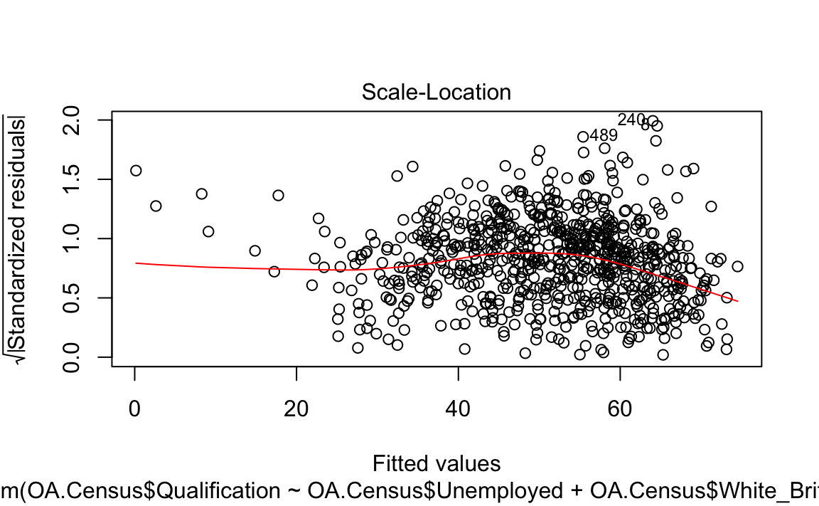
10.0.1.1 Mapping the resididuals
resids<-residuals(model)

map.resids<-OA.Census

map.resids@data <- cbind(OA.Census@data, resids)

# we need to rename the column header from the resids file - in this case its the 6th column of map.resids
names(map.resids)[6] <- "resids"

# maps the residuals using the quickmap function from tmap
qtm(map.resids, fill = "resids")
#> Variable "resids" contains positive and negative values, so midpoint is set to 0. Set midpoint = NA to show the full spectrum of the color palette.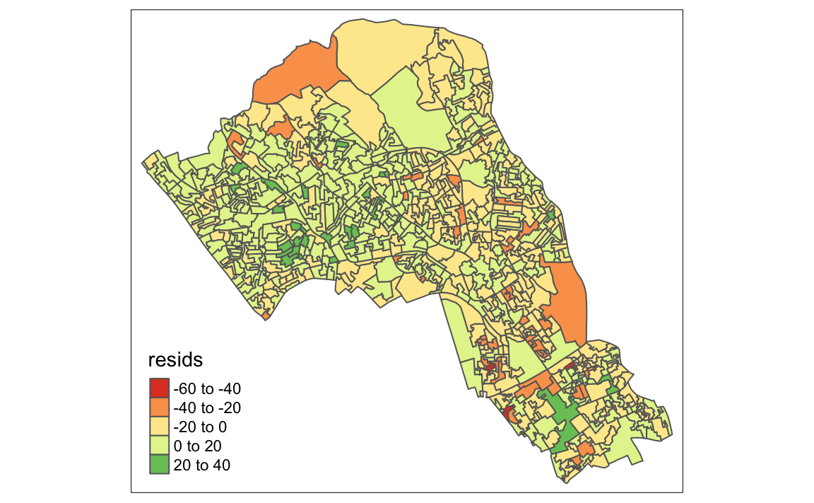
If you notice a geographic pattern to the residiuals, it is possible that an unobserved variable may also be influencing our dependent variable in the model (% with a qualification).
10.0.2 Geographically Weighted Regression (GWR)
Prior to running the model we need to calculate a kernel bandwidth. This will determine now the GWR subsets the data when its test multiple models across space.
library("spgwr")

#calculate kernel bandwidth
GWRbandwidth <- gwr.sel(OA.Census$Qualification ~ OA.Census$Unemployed+OA.Census$White_British, data=OA.Census,adapt=T)
#> Adaptive q: 0.382 CV score: 101421
#> Adaptive q: 0.618 CV score: 109723
#> Adaptive q: 0.236 CV score: 96876
#> Adaptive q: 0.146 CV score: 94192
#> Adaptive q: 0.0902 CV score: 91100
#> Adaptive q: 0.0557 CV score: 88243
#> Adaptive q: 0.0344 CV score: 85633
#> Adaptive q: 0.0213 CV score: 83790
#> Adaptive q: 0.0132 CV score: 83096
#> Adaptive q: 0.00813 CV score: 84177
#> Adaptive q: 0.0154 CV score: 83014
#> Adaptive q: 0.0152 CV score: 82957
#> Adaptive q: 0.0144 CV score: 82858
#> Adaptive q: 0.0144 CV score: 82852
#> Adaptive q: 0.0146 CV score: 82833
#> Adaptive q: 0.0148 CV score: 82855
#> Adaptive q: 0.0146 CV score: 82829
#> Adaptive q: 0.0147 CV score: 82824
#> Adaptive q: 0.0147 CV score: 82836
#> Adaptive q: 0.0147 CV score: 82824
Next we can run the model and view the results.
#run the gwr model
gwr.model = gwr(OA.Census$Qualification ~ OA.Census$Unemployed+OA.Census$White_British, data = OA.Census, adapt=GWRbandwidth, hatmatrix=TRUE, se.fit=TRUE)

#print the results of the model
gwr.model
#> Call:
#> gwr(formula = OA.Census$Qualification ~ OA.Census$Unemployed +
#>     OA.Census$White_British, data = OA.Census, adapt = GWRbandwidth,
#>     hatmatrix = TRUE, se.fit = TRUE)
#> Kernel function: gwr.Gauss
#> Adaptive quantile: 0.0147 (about 11 of 749 data points)
#> Summary of GWR coefficient estimates at data points:
#>                           Min. 1st Qu. Median 3rd Qu.   Max. Global
#> X.Intercept.            11.082  34.434 45.769  59.754 85.019  47.87
#> OA.Census.Unemployed    -5.453  -3.283 -2.554  -1.794  0.770  -3.29
#> OA.Census.White_British -0.280   0.200  0.378   0.532  0.947   0.41
#> Number of data points: 749
#> Effective number of parameters (residual: 2traceS - traceS'S): 133
#> Effective degrees of freedom (residual: 2traceS - traceS'S): 616
#> Sigma (residual: 2traceS - traceS'S): 9.9
#> Effective number of parameters (model: traceS): 94.4
#> Effective degrees of freedom (model: traceS): 655
#> Sigma (model: traceS): 9.61
#> Sigma (ML): 8.98
#> AICc (GWR p. 61, eq 2.33; p. 96, eq. 4.21): 5633
#> AIC (GWR p. 96, eq. 4.22): 5509
#> Residual sum of squares: 60452
#> Quasi-global R2: 0.73
Upon first glance, much of the outputs are identical to the outputs of the linear model. However we can explore various outputs of this model across each polygon.
We create a results output from the model which contains a number of attributes which correspond which each unique output area from our OA.Census file. In the example below we have printed the names of each of the new variables.
They include a local R2 value, the predicted values (for % qualifications) and local coefficients for each variable. We will then bind the outputs to our OA.Census polygon so we can map them.
results <-as.data.frame(gwr.model$SDF)

names(results)
#>  [1] "sum.w"                          "X.Intercept."
#>  [3] "OA.Census.Unemployed"           "OA.Census.White_British"
#>  [5] "X.Intercept._se"                "OA.Census.Unemployed_se"
#>  [7] "OA.Census.White_British_se"     "gwr.e"
#>  [9] "pred"                           "pred.se"
#> [11] "localR2"                        "X.Intercept._se_EDF"
#> [13] "OA.Census.Unemployed_se_EDF"    "OA.Census.White_British_se_EDF"
#> [15] "pred.se.1"

gwr.map<- OA.Census

gwr.map@data <- cbind(OA.Census@data, as.matrix(results))
The variable names followed by the name of our original dataframe (i.e. OA.Census.Unemployed) are the coefficients of the model.
qtm(gwr.map, fill = "localR2")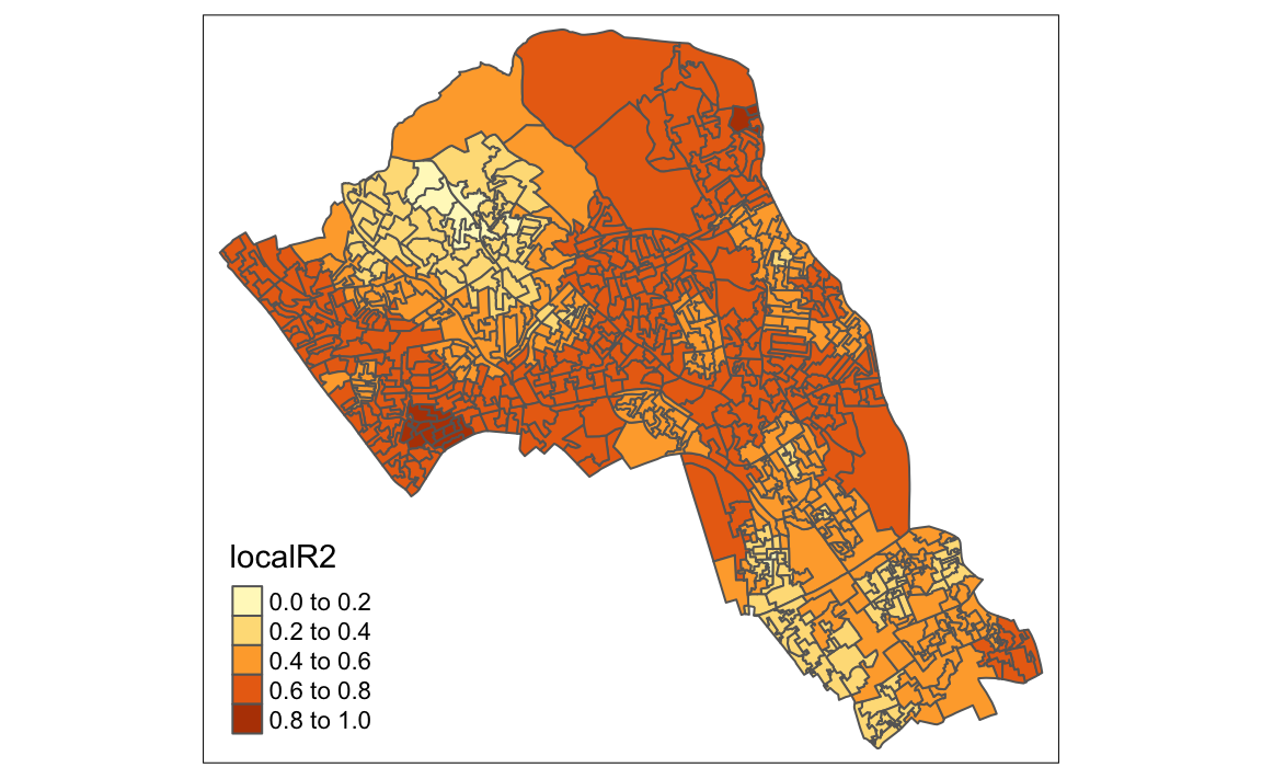
10.0.2.1 Using gridExtra
We will now consider some of the other outputs. We will create four maps in one image to show the original distributions of our unemployed and White British variables, and their coefficients in the GWR model.
To facet four maps in tmap we can use functions from the grid and gridExtra packages which allow us to split the output window into segments. We will divide the output into four and print a map in each window.
Firstly, we will create four map objects using tmap. Instead of printing them directly as we have done usually, we all assign each map an object ID so it call be called later.
# create tmap objects
map1 <- tm_shape(gwr.map) + tm_fill("White_British", n = 5, style = "quantile")  + tm_layout(frame = FALSE, legend.text.size = 0.5, legend.title.size = 0.6)
map2 <- tm_shape(gwr.map) + tm_fill("OA.Census.White_British", n = 5, style = "quantile", title = "WB Coefficient") + tm_layout(frame = FALSE, legend.text.size = 0.5, legend.title.size = 0.6)
map3 <- tm_shape(gwr.map) + tm_fill("Unemployed", n = 5, style = "quantile") + tm_layout(frame = FALSE, legend.text.size = 0.5, legend.title.size = 0.6)
map4 <- tm_shape(gwr.map) + tm_fill("OA.Census.Unemployed", n = 5, style = "quantile", title = "Ue Coefficient") + tm_layout(frame = FALSE, legend.text.size = 0.5, legend.title.size = 0.6)
With the four maps ready to be printed, we will now create a grid to print them into. From now on every time we wish to recreate the maps we will need to run the grid.newpage() function to clear the existing grid window.
library(grid)
library(gridExtra)
# creates a clear grid
grid.newpage()
# assigns the cell size of the grid, in this case 2 by 2
pushViewport(viewport(layout=grid.layout(2,2)))
# prints a map object into a defined cell
print(map1, vp=viewport(layout.pos.col = 1, layout.pos.row =1))
print(map2, vp=viewport(layout.pos.col = 2, layout.pos.row =1))
#> Variable "OA.Census.White_British" contains positive and negative values, so midpoint is set to 0. Set midpoint = NA to show the full spectrum of the color palette.
print(map3, vp=viewport(layout.pos.col = 1, layout.pos.row =2))
print(map4, vp=viewport(layout.pos.col = 2, layout.pos.row =2))
#> Variable "OA.Census.Unemployed" contains positive and negative values, so midpoint is set to 0. Set midpoint = NA to show the full spectrum of the color palette.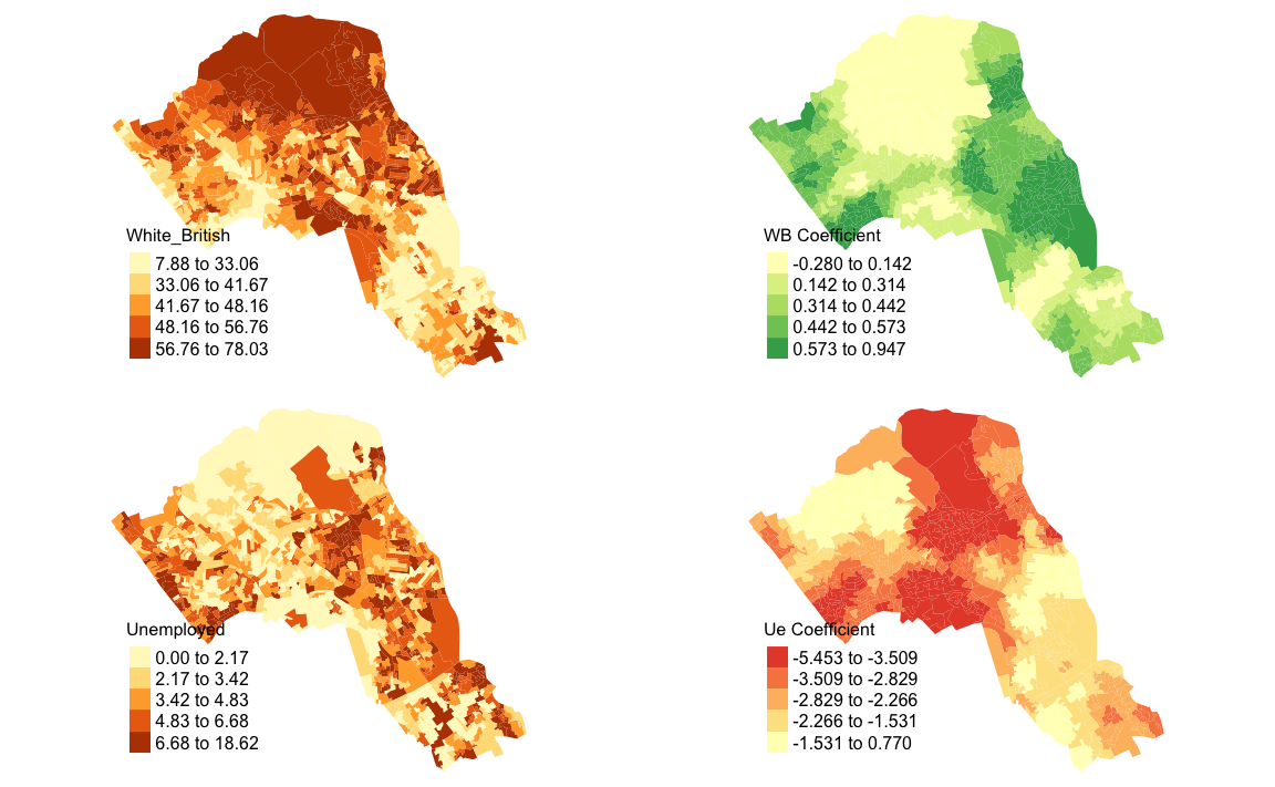 ##Additional Task
Write a 350 word summary of the above results. Comment on the value of GWR in this context and suggest additional methods that may also be appropriate. Print this and bring to the next lecture.