16 Further techniques in linear regression’
16.1 Dealing with non linearities
Is the relationship between body mass index and age linear? If we were to fit a model and test the assumptions covered in Week 9 of POLS0008, we would would find that the residual plots indicate that the bmi on age model we fit underpredicts at younger and, particularly, older ages. Let’s look at the bivariate relationship between these two variables through a scatterplot. You will need to load the 2012_hse_and_shes_combined.dta file into your workspace before you start.
library(foreign)
hse_and_shes12 <- read.dta("worksheet_data/regression/2012_hse_and_shes_combined.dta")
library(ggplot2)
ggplot(hse_and_shes12, aes(x=age, y=bmival)) +
geom_point(shape=1) 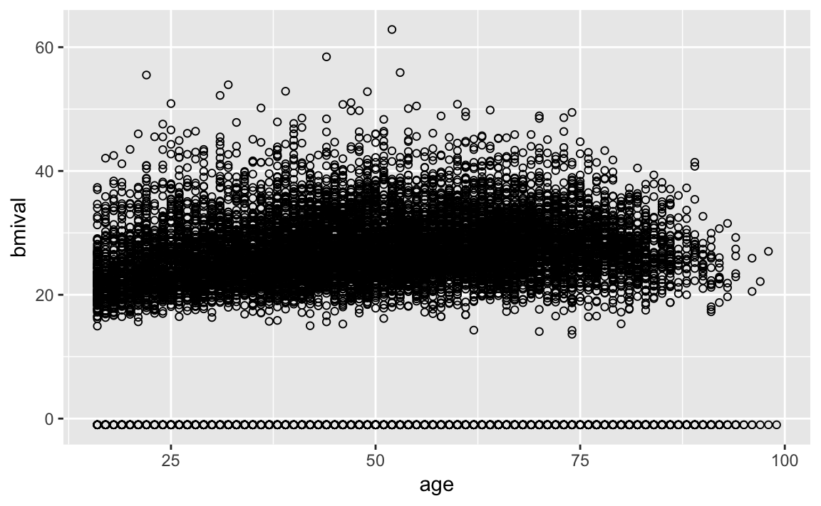
What do you immediately notice about this plot? Probably not the non-linear relationship between age and BMI, but the large number of cases that have BMI values below zero. These are respondents who have we are not able to calcualte a BMI value for because they did not provide height and/or weight measurements, or these measurements were invalid. In these data, these respondents have been given a value of -1. It is common in large sample survey datasets for missing values to be given values below zero to indicate to the analyst that they are missing. Value from -999 to -1 are often used to indicate the nature of the missingness (e.g. item not applicable, respondents refused to answer, etc). We will cover missing data in more detail in Week 10.
For now we will simply discard respondents who do not have a valid BMI value and also exclude anyone aged below 18 because BMI is calculated differently for children.
hse_and_shes12.subset<-subset(hse_and_shes12, bmival>0 & age>=18) As we said one of the fundamental assumptions of linear regression is that the model assumes that a straight line is a good representation of the data. If this is not the case you may better off using some form of nonlinear model. So, one of the first things you want to do when looking at your data is to assess if a straight line represents a reasonable summary for it. Let’s fit a model only including Age as an explanatory variable using ggplot.
library(ggplot2)
ggplot(hse_and_shes12.subset, aes(x=age, y=bmival)) +
    geom_point(shape=1) +
geom_smooth(method = "lm") 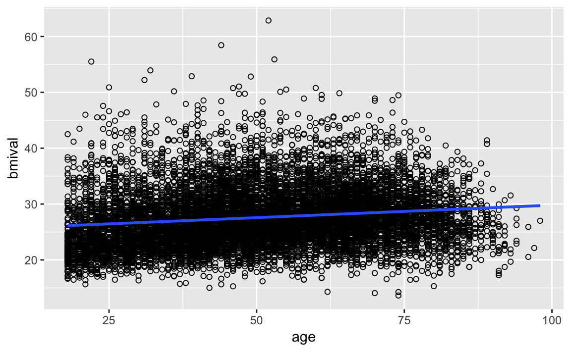
Is the straight line a good summary?
We already knew from the residual plots we had a problem here, but hopefully this plot also helps you to see the problem more clearly. This plot seems to suggest that perhaps the relationship here is somehow curvilinear.
What do you do in a situation such as this? There are a number of solutions, some of which are more complex than others. One fairly simple way of extending the linear model is by using polynomial regression. Essentially what this does is to incorporate a transformed predictor into the model with the intention of capturing the curvature apparent in the data. What we do is that we add additional terms to the model until we are satisfied we capture the pattern in the data.
So say we are working with a simple model of bmival ~ Age. We could try to fit a polynomial regression adding a second term with a squared Age. This would produce the following predicted line:
#We are asking ggplot to produce a linear model using the specified formula. This formula asks for a polynomial regression with a quadratic term added (that's why you see the I(x^2)).
ggplot(hse_and_shes12.subset, aes(x=age, y=bmival)) +
  geom_point() +
  geom_smooth(method = "lm", formula = y ~ x + I(x^2)) #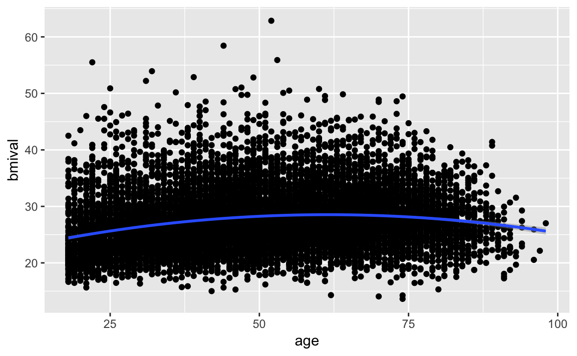
Essentially, adding this extra term allows the possibility of a decreasing slope with Age and helps to model an inverted U-shaped pattern. If we still think that the non-linearities are not adequately captured we could try with a cubic transformation (raising to the power of 3) and adding this additional term. The more complex your polynomial, the more difficult it may be to interpret your tabular results.
Let’s return to the more complex model we were examining the differences by Age and Sex and run the model with a quadratic Age term added, starting by fitting a model without the quadratic. We will also add Sex to our model given the differences expected between men and women.
bmi.model <- lm(bmival~age+Sex, data=hse_and_shes12.subset)
summary(bmi.model)
#>
#> Call:
#> lm(formula = bmival ~ age + Sex, data = hse_and_shes12.subset)
#>
#> Residuals:
#>    Min     1Q Median     3Q    Max
#> -15.20  -3.62  -0.73   2.74  35.36
#>
#> Coefficients:
#>             Estimate Std. Error t value Pr(>|t|)
#> (Intercept) 25.54663    0.16374  156.02  < 2e-16 ***
#> age          0.04444    0.00285   15.59  < 2e-16 ***
#> SexFemale   -0.36192    0.10109   -3.58  0.00034 ***
#> ---
#> Signif. codes:  0 '***' 0.001 '**' 0.01 '*' 0.05 '.' 0.1 ' ' 1
#>
#> Residual standard error: 5.21 on 10715 degrees of freedom
#> Multiple R-squared:  0.0236, Adjusted R-squared:  0.0234
#> F-statistic:  129 on 2 and 10715 DF,  p-value: <2e-16
bmi.modelq <- lm(bmival~age+I(age^2)+Sex, data=hse_and_shes12.subset)
summary(bmi.modelq)
#>
#> Call:
#> lm(formula = bmival ~ age + I(age^2) + Sex, data = hse_and_shes12.subset)
#>
#> Residuals:
#>    Min     1Q Median     3Q    Max
#> -14.74  -3.54  -0.72   2.69  34.67
#>
#> Coefficients:
#>              Estimate Std. Error t value Pr(>|t|)
#> (Intercept) 20.525240   0.386501   53.11  < 2e-16 ***
#> age          0.266521   0.015771   16.90  < 2e-16 ***
#> I(age^2)    -0.002169   0.000152  -14.31  < 2e-16 ***
#> SexFemale   -0.336077   0.100157   -3.36  0.00079 ***
#> ---
#> Signif. codes:  0 '***' 0.001 '**' 0.01 '*' 0.05 '.' 0.1 ' ' 1
#>
#> Residual standard error: 5.16 on 10714 degrees of freedom
#> Multiple R-squared:  0.0419, Adjusted R-squared:  0.0416
#> F-statistic:  156 on 3 and 10714 DF,  p-value: <2e-16
The near-zero p-value associated with the quadratic Age term suggests that it leads to an improved model. We can use the anova() function to quantify the improvement in the model.
anova(bmi.model, bmi.modelq)
#> Analysis of Variance Table
#>
#> Model 1: bmival ~ age + Sex
#> Model 2: bmival ~ age + I(age^2) + Sex
#>   Res.Df    RSS Df Sum of Sq   F Pr(>F)
#> 1  10715 290636
#> 2  10714 285183  1      5453 205 <2e-16 ***
#> ---
#> Signif. codes:  0 '***' 0.001 '**' 0.01 '*' 0.05 '.' 0.1 ' ' 1
In the output the first model is the one without the quadratic term (the straight line model) and the second model is the one with the added polynomial. What the anova() function is doing here is to run a hypothesis test that the two models fit the data equally well, whereas the research hypothesis is that the model with the quadratic term represents a better fit. The p value we observe is zero. So clearly in this case adding a quadratic term represents an improvement to our model. If we compare the plot of the residuals against the fitted values we can see that the non-linear pattern that was evident in our simpler model washes away once we introduce the quadratic term.
#You would use this code to obtain only the fitted against the residuals
library(car)
residualPlots(bmi.model, ~1, fitted = TRUE)
#>            Test stat Pr(>|Test stat|)
#> Tukey test     -12.4           <2e-16 ***
#> ---
#> Signif. codes:  0 '***' 0.001 '**' 0.01 '*' 0.05 '.' 0.1 ' ' 1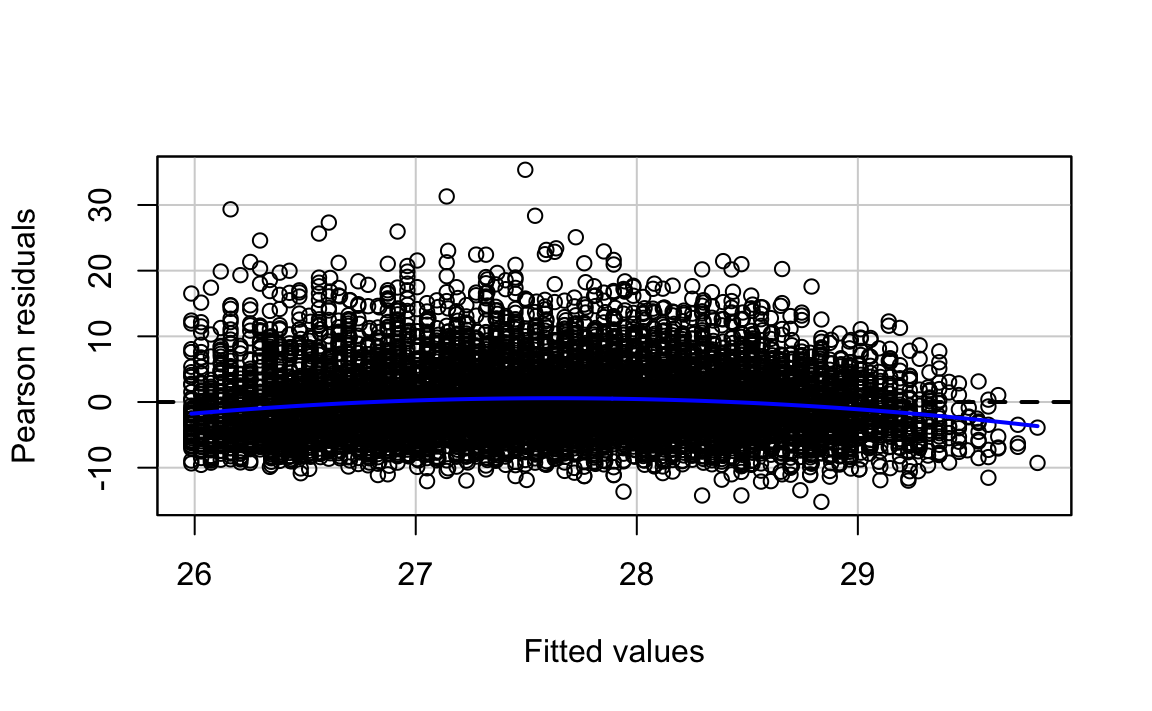
residualPlots(bmi.modelq, ~1, fitted = TRUE)
#>            Test stat Pr(>|Test stat|)
#> Tukey test      0.94             0.35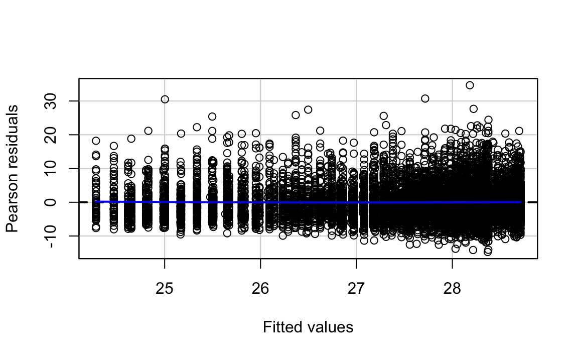
We can see that the Tukey test is no longer significant. But should we add a cubic term?
bmi.modelc <- lm(bmival~age+I(age^2)+I(age^3)+Sex, data=hse_and_shes12.subset)
summary(bmi.modelc)
#>
#> Call:
#> lm(formula = bmival ~ age + I(age^2) + I(age^3) + Sex, data = hse_and_shes12.subset)
#>
#> Residuals:
#>    Min     1Q Median     3Q    Max
#> -14.78  -3.55  -0.73   2.71  34.67
#>
#> Coefficients:
#>              Estimate Std. Error t value Pr(>|t|)
#> (Intercept)  2.18e+01   9.22e-01   23.70  < 2e-16 ***
#> age          1.74e-01   6.08e-02    2.86  0.00422 **
#> I(age^2)    -2.34e-04   1.23e-03   -0.19  0.84932
#> I(age^3)    -1.24e-05   7.83e-06   -1.58  0.11422
#> SexFemale   -3.30e-01   1.00e-01   -3.29  0.00099 ***
#> ---
#> Signif. codes:  0 '***' 0.001 '**' 0.01 '*' 0.05 '.' 0.1 ' ' 1
#>
#> Residual standard error: 5.16 on 10713 degrees of freedom
#> Multiple R-squared:  0.0421, Adjusted R-squared:  0.0418
#> F-statistic:  118 on 4 and 10713 DF,  p-value: <2e-16
In this case, we have less evidence that adding this additional term would improve the fit. As you can see the p value associated with the cubic term is not significant.
As we discussed when introducing regression, interpreting the coefficients can get tricky. That is certainly the case when you add polynomial regression. The description of results in this case will typically focus on the general pattern of results, rather than in the regression coefficients for your transformed variable. One solution to this is to produce graphical displays of the relationship such as those that can be obtained with the effects package.
library(effects)
plot(allEffects(bmi.modelq)$age)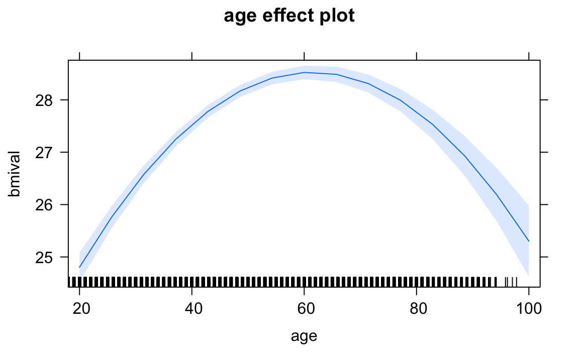
We have discussed transforming the variable by squaring it, but other curvilinear patterns may require other transformations such as taking the inverse (1/X), when there is a decreasing negative effect of the predictor on the response variable, or taking the square root of X, when there is a diminishing positive impact of the predictor on the response variable. There are also other more sophisticated ways of accommodating non linearities by means of fitting regression splines or using generalised additive models.
16.2 Transformations
You may have noticed in the residual plot for our polynomial regression that the variance still does not seem constant when looking at the fitted values. Again, there are a number of solutions one could apply in this type of scenarios. Check your notes from POLS0008 for code to replace the usual coefficient standard errors with standard errors that will be consistent even with heterokedasticity.
Let’s look at another example using the election17aps17 dataset. We will model the Liberal Democrat proportion of vote (ld.per) in a parliamentary constituency as a linear function of percentage of White ethnic group residents (White), percentage employed as managers (Manager), and dummy variables for the region (region).
Before we do we must correct a “problem” in the dataset. The parliamentry seats of Skipton and Ripon and Brighton Pavilion were not contested by the Liberal Democrats because the party stood aside and endorsed the Green party for these seats. At present, a value for the percentage of votes to the Lib Dems is 0% in election17aps17, which is factually correct. However, given they didn’t contest the seat it makes sense to remove this row from the analysis. We will do this by simply assigning a missing value to the ld.per variable for these constituencies. What implication does this have on our ability to generalise to a wider population?
election17aps17$ld.per[election17aps17$ld.per==0] <- NA
ld.model <- lm(ld.per~White+Manager+region_name, data=election17aps17)
summary(ld.model)
#>
#> Call:
#> lm(formula = ld.per ~ White + Manager + region_name, data = election17aps17)
#>
#> Residuals:
#>     Min      1Q  Median      3Q     Max
#> -0.1244 -0.0378 -0.0181  0.0046  0.4185
#>
#> Coefficients:
#>                                      Estimate Std. Error t value Pr(>|t|)
#> (Intercept)                         -0.054939   0.031069   -1.77    0.078
#> White                                0.000736   0.000331    2.22    0.026
#> Manager                              0.005376   0.000941    5.71  1.7e-08
#> region_nameEast Midlands            -0.023048   0.015976   -1.44    0.150
#> region_nameLondon                    0.026551   0.016955    1.57    0.118
#> region_nameNorth East               -0.016491   0.018690   -0.88    0.378
#> region_nameNorth West               -0.012049   0.014187   -0.85    0.396
#> region_nameScotland                  0.008871   0.015332    0.58    0.563
#> region_nameSouth East                0.025862   0.013813    1.87    0.062
#> region_nameSouth West                0.069443   0.015203    4.57  6.0e-06
#> region_nameWales                    -0.021967   0.016809   -1.31    0.192
#> region_nameWest Midlands            -0.019617   0.015108   -1.30    0.195
#> region_nameYorkshire and The Humber -0.013206   0.015544   -0.85    0.396
#>
#> (Intercept)                         .
#> White                               *
#> Manager                             ***
#> region_nameEast Midlands
#> region_nameLondon
#> region_nameNorth East
#> region_nameNorth West
#> region_nameScotland
#> region_nameSouth East               .
#> region_nameSouth West               ***
#> region_nameWales
#> region_nameWest Midlands
#> region_nameYorkshire and The Humber
#> ---
#> Signif. codes:  0 '***' 0.001 '**' 0.01 '*' 0.05 '.' 0.1 ' ' 1
#>
#> Residual standard error: 0.0804 on 614 degrees of freedom
#>   (5 observations deleted due to missingness)
#> Multiple R-squared:  0.191,  Adjusted R-squared:  0.175
#> F-statistic: 12.1 on 12 and 614 DF,  p-value: <2e-16
We see that the R square is not too bad at .1954 and all of the explanatory variables are significantly associated with percentage of votes for Liberal Democrat candidate in the direction one might expect. Do you agree? Constituencies with a higher proportion of White ethnic group residents and residents employed as managers tend to give proportionately more votes proportionally to a Liberal Democrat candidate. The regional dummy variables show that compared with constituencies in the East region, constituencies in the South West region are more likely to have a higher proportion of the vote going to Liberal Democrat candidates.
residualPlots(ld.model)
#>             Test stat Pr(>|Test stat|)
#> White           -0.20           0.8385
#> Manager          0.20           0.8402
#> region_name
#> Tukey test       2.64           0.0082 **
#> ---
#> Signif. codes:  0 '***' 0.001 '**' 0.01 '*' 0.05 '.' 0.1 ' ' 1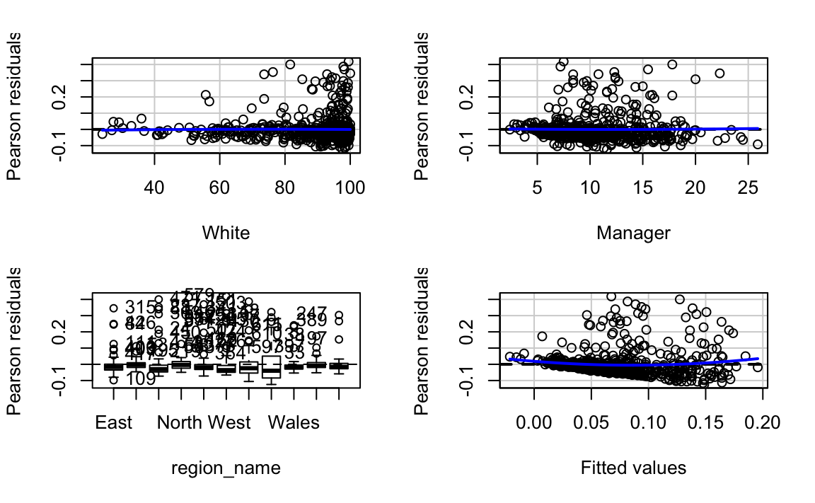
We can see minor non-linearities and more obvious unequal variances when plotting the residuals against the fitted values and each explanatory variables. And if we were to look at outliers we would also see problems.
outlierTest(ld.model)
#>     rstudent unadjusted p-value Bonferroni p
#> 584     5.37           1.14e-07     7.14e-05
#> 476     5.13           3.88e-07     2.43e-04
#> 155     4.95           9.66e-07     6.06e-04
#> 508     4.72           2.98e-06     1.87e-03
#> 241     4.50           8.17e-06     5.12e-03
#> 319     4.43           1.12e-05     7.01e-03
#> 92      4.32           1.83e-05     1.15e-02
#> 345     4.32           1.85e-05     1.16e-02
#> 18      4.09           4.84e-05     3.04e-02
#> 551     4.00           7.06e-05     4.42e-02
A few of the outliers are significant and the influence plot shows further evidence of it:
influencePlot(ld.model)
#>     StudRes    Hat   CookD
#> 35    0.559 0.0670 0.00173
#> 253   0.609 0.0854 0.00267
#> 319   4.430 0.0312 0.04718
#> 476   5.131 0.0209 0.04147
#> 584   5.367 0.0174 0.03759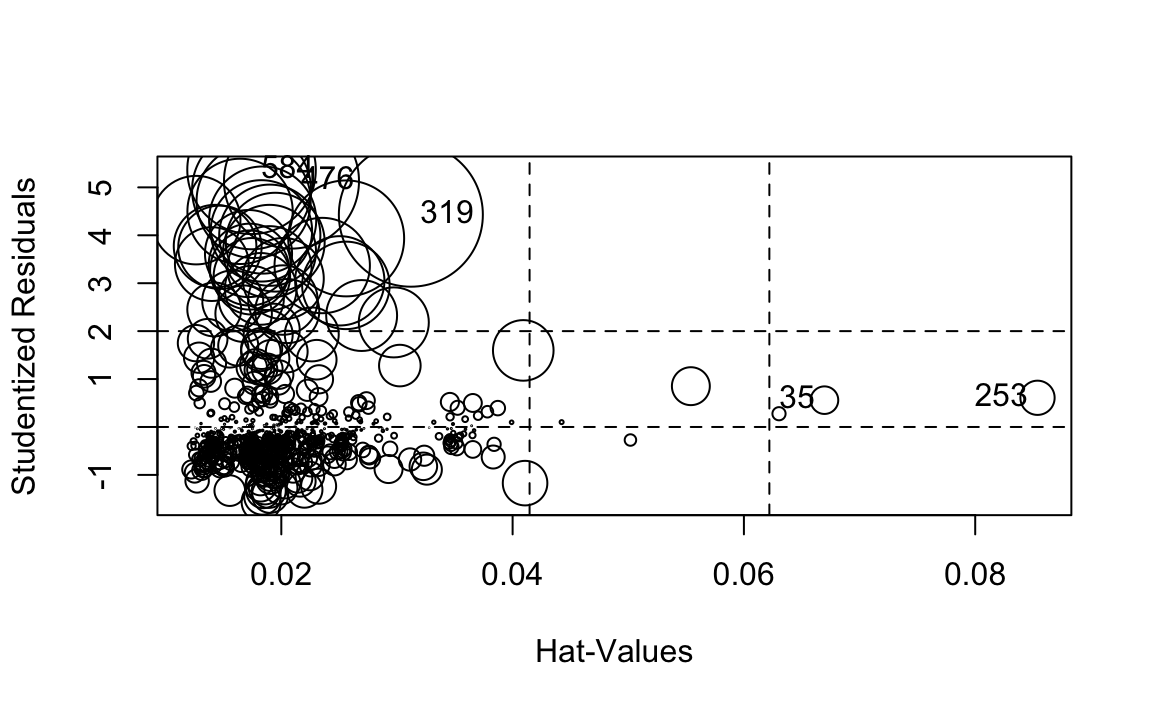
What this analysis shows is that often problems come together and are related to each other. If you have plotted the distribution of ld.per you will see it is positively skewed. In these cases it can make sense to transform the Y variable as a first step, since this skew is likely to be playing a role in the unequal spread that we see in the residual plots.
We can use the symbox() function from the car package to investigate what transformation will make ld.per less skewed.
symbox(~ld.per, data=election17aps17, na.rm=TRUE)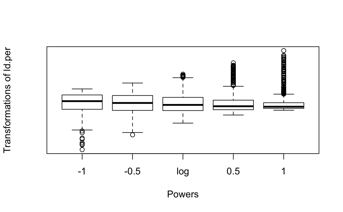
This set of boxplots suggests what the distribution of ld.per would look like if we were to apply different power transformations. In this case, as in many other instances with skewed distributions, applying the logarithmic transformation seems the most appropriate one. Let’s explore the implications of it:
ld.logmodel <- lm(log(ld.per)~White+Manager+region_name, data=election17aps17)
summary(ld.logmodel)
#>
#> Call:
#> lm(formula = log(ld.per) ~ White + Manager + region_name, data = election17aps17)
#>
#> Residuals:
#>     Min      1Q  Median      3Q     Max
#> -1.5748 -0.4593 -0.0977  0.3068  2.5025
#>
#> Coefficients:
#>                                     Estimate Std. Error t value Pr(>|t|)
#> (Intercept)                         -4.48351    0.27417  -16.35  < 2e-16
#> White                                0.00783    0.00292    2.68   0.0075
#> Manager                              0.07303    0.00830    8.79  < 2e-16
#> region_nameEast Midlands            -0.27339    0.14098   -1.94   0.0529
#> region_nameLondon                    0.16938    0.14962    1.13   0.2581
#> region_nameNorth East               -0.23969    0.16493   -1.45   0.1466
#> region_nameNorth West               -0.31855    0.12520   -2.54   0.0112
#> region_nameScotland                 -0.06747    0.13530   -0.50   0.6182
#> region_nameSouth East                0.32677    0.12190    2.68   0.0075
#> region_nameSouth West                0.61863    0.13416    4.61  4.9e-06
#> region_nameWales                    -0.55491    0.14833   -3.74   0.0002
#> region_nameWest Midlands            -0.33446    0.13332   -2.51   0.0124
#> region_nameYorkshire and The Humber -0.29635    0.13717   -2.16   0.0311
#>
#> (Intercept)                         ***
#> White                               **
#> Manager                             ***
#> region_nameEast Midlands            .
#> region_nameLondon
#> region_nameNorth East
#> region_nameNorth West               *
#> region_nameScotland
#> region_nameSouth East               **
#> region_nameSouth West               ***
#> region_nameWales                    ***
#> region_nameWest Midlands            *
#> region_nameYorkshire and The Humber *
#> ---
#> Signif. codes:  0 '***' 0.001 '**' 0.01 '*' 0.05 '.' 0.1 ' ' 1
#>
#> Residual standard error: 0.71 on 614 degrees of freedom
#>   (5 observations deleted due to missingness)
#> Multiple R-squared:  0.331,  Adjusted R-squared:  0.318
#> F-statistic: 25.4 on 12 and 614 DF,  p-value: <2e-16
You will notice that the coefficients change in magnitude, since we have re-expressed the response variable in the logarithmic scale, but the direction and the statistical significance remain unchanged. The R square, however, is better. Let’s look at the residuals:
residualPlots(ld.logmodel)
#>             Test stat Pr(>|Test stat|)
#> White           -0.96             0.34
#> Manager         -0.08             0.93
#> region_name
#> Tukey test       1.07             0.28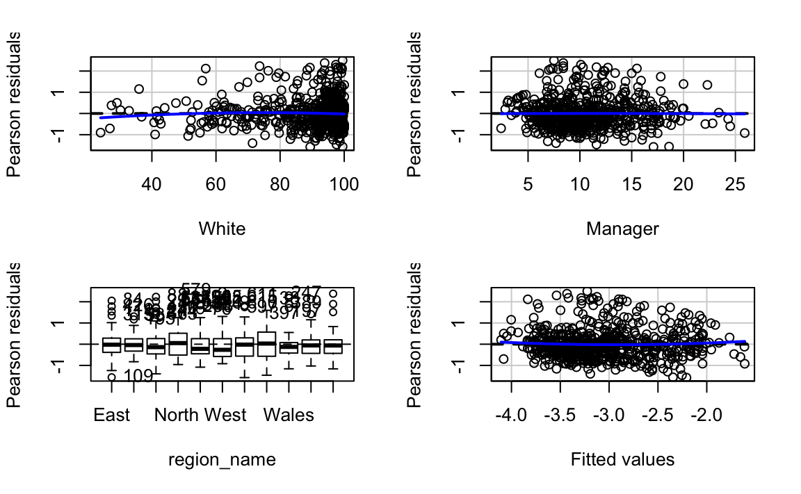
We can see that the non-constant variance is still present, though to a lesser degree. We can further investigate this model using plots compare the distribution and relationship of the variables in our model. In fact, this should typically precede fitting the model to assess potential non-linearities, outliers and skewed distributions. We will use the scatterplotMatrix of the car package.
scatterplotMatrix(~ log(ld.per) + White + Manager + region_name, data=election17aps17)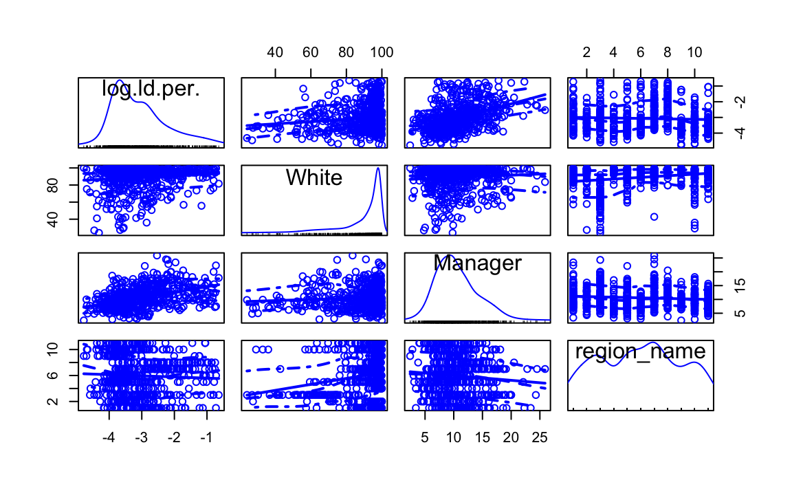
The matrix reveals that the distributions of the White predictor is all also suffering from some skew. A solution in this case is to try transformations of the explanatory variables.
ld.loglogmodel <- lm(log(ld.per)~log(White)+Manager+region_name, data=election17aps17)
summary(ld.loglogmodel)
#>
#> Call:
#> lm(formula = log(ld.per) ~ log(White) + Manager + region_name,
#>     data = election17aps17)
#>
#> Residuals:
#>    Min     1Q Median     3Q    Max
#> -1.582 -0.460 -0.100  0.298  2.510
#>
#> Coefficients:
#>                                     Estimate Std. Error t value Pr(>|t|)
#> (Intercept)                         -6.19630    0.84579   -7.33  7.5e-13
#> log(White)                           0.53858    0.19093    2.82  0.00495
#> Manager                              0.07296    0.00828    8.82  < 2e-16
#> region_nameEast Midlands            -0.26862    0.14088   -1.91  0.05703
#> region_nameLondon                    0.16211    0.14600    1.11  0.26730
#> region_nameNorth East               -0.23177    0.16437   -1.41  0.15903
#> region_nameNorth West               -0.31813    0.12511   -2.54  0.01124
#> region_nameScotland                 -0.06017    0.13472   -0.45  0.65532
#> region_nameSouth East                0.32793    0.12182    2.69  0.00730
#> region_nameSouth West                0.62555    0.13383    4.67  3.6e-06
#> region_nameWales                    -0.54660    0.14778   -3.70  0.00024
#> region_nameWest Midlands            -0.33289    0.13322   -2.50  0.01272
#> region_nameYorkshire and The Humber -0.29605    0.13707   -2.16  0.03117
#>
#> (Intercept)                         ***
#> log(White)                          **
#> Manager                             ***
#> region_nameEast Midlands            .
#> region_nameLondon
#> region_nameNorth East
#> region_nameNorth West               *
#> region_nameScotland
#> region_nameSouth East               **
#> region_nameSouth West               ***
#> region_nameWales                    ***
#> region_nameWest Midlands            *
#> region_nameYorkshire and The Humber *
#> ---
#> Signif. codes:  0 '***' 0.001 '**' 0.01 '*' 0.05 '.' 0.1 ' ' 1
#>
#> Residual standard error: 0.709 on 614 degrees of freedom
#>   (5 observations deleted due to missingness)
#> Multiple R-squared:  0.332,  Adjusted R-squared:  0.319
#> F-statistic: 25.5 on 12 and 614 DF,  p-value: <2e-16
Transforming the White variable in the logarithmic scale, however, does not seem to increase the R square and therefore we should use the original variables to make the model easier to interpret. You could try and alternative transformation. Remember that any transformation has implications for how you can interpret your model. Another solution is to recode these skewed variables into categorical predictors that represent the majority of compared with the minority of extreme values (e.g. <10% ethnic minorities, 10-20% ethnic minorities, 20%+ ethnic minorities) and then add these to the model.
16.3 Interactions
In the social sciences there is a great interest in what are called conditional hypothesis or interactions. Many of our theories do not assume simply additive effects but multiplicative effects.
One of the assumptions of the regression model is that the relationship between the response variable and your predictors is additive. That is, if you have two predictors x1 and x2. Regression assumes that the effect of x1 on y is the same at all levels of x2. If that is not the case, you are then violating one of the assumptions of regression. This is in fact one of the most important assumptions of regression, even if researchers often overlook it.
One way of extending our model to accommodate for interaction effects is to add additional terms to our model, a third predictor x3, where x3 is simply the product of multiplying x1 by x2. Notice we keep a term for each of the main effects (the original predictors) as well as a new term for the interaction effect.
Let’s return to the hse_and_shes12 dataset and consider the relationship between mental wellbeing and bmi and sex. We might have cause to believe that wellbeing differs over bmi in men compared with women. Perhaps there is something associated with having a higher bmi that causes women lower wellbeing that doesn’t affect men to the same extent because of some third variable (e.g. marriage).
How do we test this in R? The easiet way to add an interaction term in R is to add a multiplication sign between the two variables you want to interact. The following example is asking R to test the conditional hypothesis that the bmi may have a different impact on mental wellbeing (wemwbs) for men and women. We will need to remove missing values of wemwbs from our hse_and_shes12.subset dataset.
hse_and_shes12.subset1<-subset(hse_and_shes12.subset, wemwbs>=0)
wemwbs.model <- lm(wemwbs~bmival*Sex, data=hse_and_shes12.subset1)
summary(wemwbs.model)
#>
#> Call:
#> lm(formula = wemwbs ~ bmival * Sex, data = hse_and_shes12.subset1)
#>
#> Residuals:
#>    Min     1Q Median     3Q    Max
#> -38.33  -5.41   0.84   5.59  21.38
#>
#> Coefficients:
#>                  Estimate Std. Error t value Pr(>|t|)
#> (Intercept)       53.3055     0.9142   58.31   <2e-16 ***
#> bmival            -0.0583     0.0323   -1.80    0.071 .
#> SexFemale          2.0195     1.1216    1.80    0.072 .
#> bmival:SexFemale  -0.0917     0.0398   -2.31    0.021 *
#> ---
#> Signif. codes:  0 '***' 0.001 '**' 0.01 '*' 0.05 '.' 0.1 ' ' 1
#>
#> Residual standard error: 8.87 on 8065 degrees of freedom
#> Multiple R-squared:  0.00626,    Adjusted R-squared:  0.00589
#> F-statistic: 16.9 on 3 and 8065 DF,  p-value: 5.72e-11
You see here that essentially you have only two inputs (bmi and sex) but several regression coefficients. Gelman and Hill (2007) suggest reserving the term input for the variables encoding the information and to use the term predictor to refer to each of the terms in the model. So here we have two inputs and four predictors (one for the constant term, one for bmi, another for sex, and a final one for the interaction term).
What we see here is that the interaction included is significant. To assist interpretation of interactions is helpful to look at effect plots. Let’s visualise the results with the effects package:
plot(effect("bmival:Sex", wemwbs.model))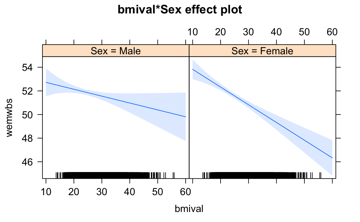
I said above that the interaction may not be instrincally related to sex, but something that else that protects men with a higher bmi value from having lower mental wellbeing (e.g. marriage). What happens if we add marital status (maritalg) to the model? Try it. You should remove the categories/levels Don't know and Refused. Is the interaction significant when included marital status in the model?
16.4 Acknowledgements
This exercise was adapted from R for Criminologists developed by Juanjo Medina and is licensed under a Creative Commons Attribution-Non Commercial 4.0 International License.
16.5 Additional Exercise
Using the
hse_and_shes12dataset, fit a model predictingwemwbsincluding equivalised incomeeqvincand two other variables of your choice. Test for non-linear relationships between mental wellbeing and income. Interpret the results.Using the
election17aps17dataset, run a multiple regression onukip.per, the percent of votes for a UK Indepedence Party candidate, including up to four explanatory variables of your choice. Interpret the results and explain whether you consider transforming any variables in your model.Going back to the
hse_and_shes12dataset, fit a model predicting body mass index,bmivaladding equivalised incomeeqvincand sex as input variables. Add an interaction term between income and sex. Interpret the results.