6 Mapping Point Data in R

In this practical we will: * Create a point shapefile form a csv using coordinates * Map the points in tmap * Create a proportion bubble map

First we must make sure that our working directory is set and then we can load in our data.

# Load the data. You may need to alter the file directory
Census.Data <-read.csv("worksheet_data/camden/practical_data.csv")

We will also need the polygon shapefile from our previous exercise and join our census data to it.

# load the spatial libraries
library("rgdal")
library("rgeos")
# Load the output area shapefiles
Output.Areas <- readOGR("worksheet_data/camden", "Camden_oa11")
#> OGR data source with driver: ESRI Shapefile 
#> Source: "/Users/jamestodd/Desktop/GitHub/learningR/worksheet_data/camden", layer: "Camden_oa11"
#> with 749 features
#> It has 1 fields

# join our census data to the shapefile
OA.Census <- merge(Output.Areas, Census.Data, by.x="OA11CD", by.y="OA")

6.0.1 Loading point data into R

In this practical we will be handling house price paid data originally made available for free by the Land Registry. You can download a version of the data from HERE. The data is formatted as CSV where each row is a unique house sale, including the price paid in pounds and the postcode. Prior to this practical, the data file was joined to a Office for National Statistics (ONS) postcode lookup table which allows us to join the x and y and ONS geographic units for each postcode.

# load the house prices csv file
houses <- read.csv("worksheet_data/camden/CamdenHouseSales15.csv")
# we only need a few columns for this practical
houses <- houses[,c(1,2,8,9)]

Whilst it is possible to plot this data using the standard plot() in R. It is not being handled as spatial data as demonstrated below.

# 2D scatter plot
plot(houses$oseast1m, houses$osnrth1m)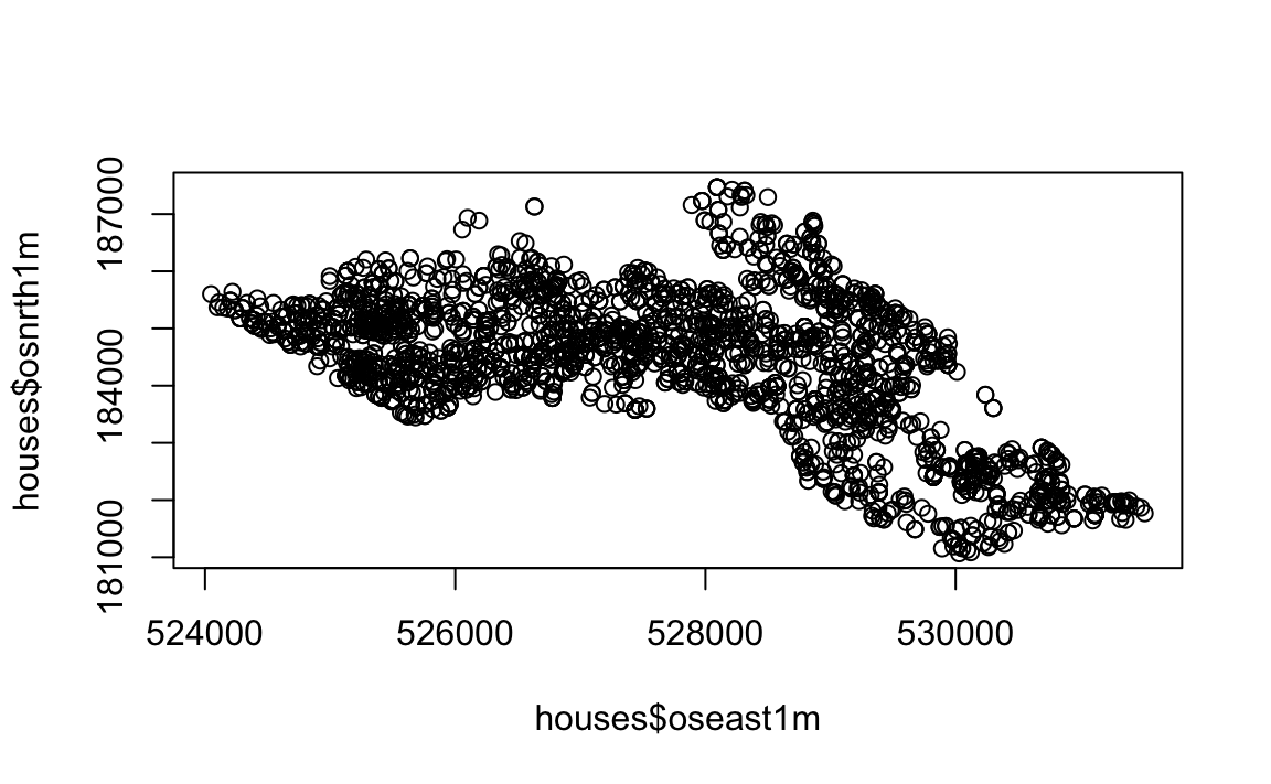

Therefore, we need to assign spatial attributes to the CSV so it can be mapped properly in R. To do this we will need to load the sp package in r, this package provides classes and methods for handling spatial data. Remember to install the package first if you have not done so before. Next we will convert the csv into a SpatialPointsDataFrame. To do this we will need to set what the data is to be included, what columns contain the x and y coordinates, and what projection system we are using.

library("sp")
# create a House.Points SpatialPointsDataFrame. Note how the houses[,3:4] part of the code
# is extracting the coordinates we need. "houses" specifies the data object we could like
# to append the coordinates to and our proj4string sets the coordinate projection system.
House.Points <-SpatialPointsDataFrame(houses[,3:4], houses, proj4string = CRS("+init=epsg:27700"))

Before we map the points, we will first create a base map using the output area boundaries.

library("tmap")
# This plots a blank base map, we have set the transparency of the borders to 0.4
tm_shape(OA.Census) + tm_borders(alpha=.4)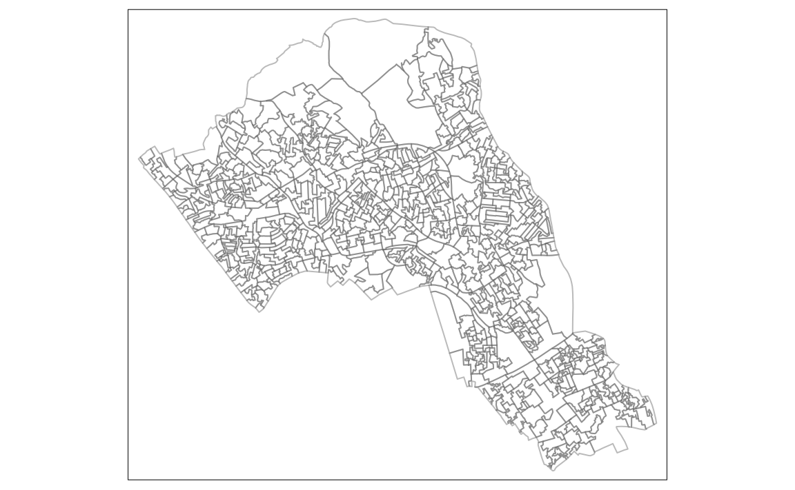

We can now add on the points as an additional tm_shape in our map. So here, we copy in the same code to make the base map, add on a plus symbol, then enter the details for the points data. The additional arguments for the points data can be summarised as:

tm_shape(polygon file) + tm_borders(transparency = 40%) + tm_shape(our spatial points data frame) + tm_dots(what variable is coloured, the colour palette and interval style) Which is entered into R like this:

# creates a coloured dot map
tm_shape(OA.Census) + tm_borders(alpha=.4) +
tm_shape(House.Points) + tm_dots(col = "Price", palette = "Reds", style = "quantile")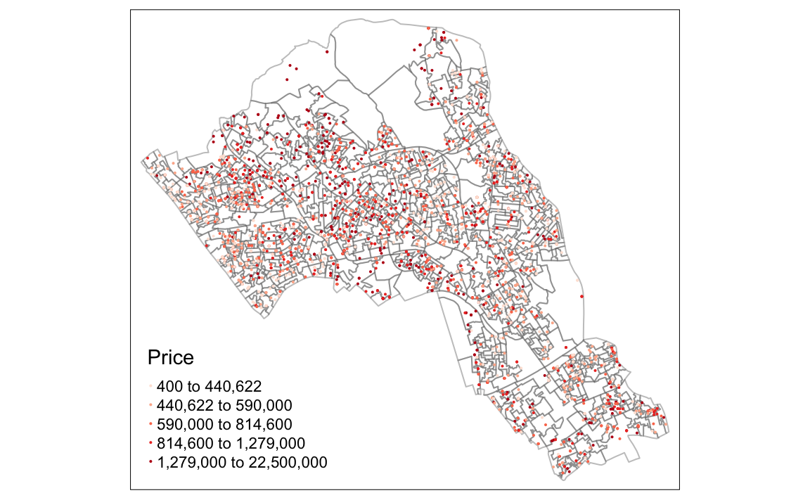

We can also add in more arguments within the tm_dots() function for points like we would with tm_fill() for polygon data. Some arguments are unique to tm_dots(), for example the option t

# creates a coloured dot map
tm_shape(OA.Census) + 
  tm_borders(alpha=.4) +
  tm_shape(House.Points) + 
  tm_dots(col = "Price", scale = 1.5, palette = "Reds", style = "quantile", title = "Price Paid (?)")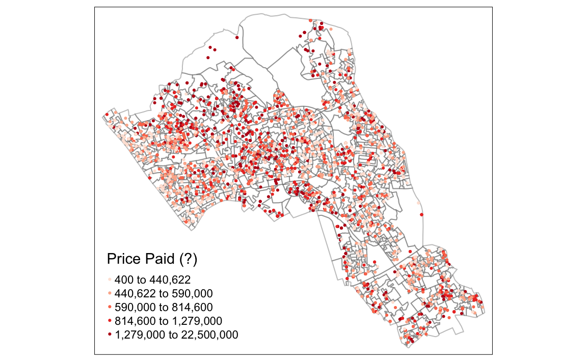

We can also add tm_layout() and tm_compass() as we did in the previous practical.

# creates a coloured dot map
tm_shape(OA.Census) + 
  tm_borders(alpha=.4) +
  tm_shape(House.Points) + 
  tm_dots(col = "Price", scale = 1.5, palette = "Purples", style = "quantile", title = "Price Paid (?)") +
  tm_compass() +
  tm_layout(legend.text.size = 1.1, legend.title.size = 1.4, frame = FALSE)
#> Some legend labels were too wide. These labels have been resized to 0.92, 0.92, 0.84, 0.74. Increase legend.width (argument of tm_layout) to make the legend wider and therefore the labels larger.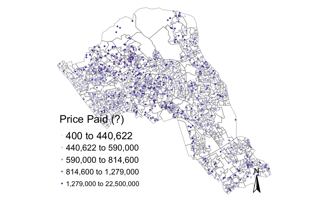

Some legend labels were too wide. These labels have been resized to 0.93. Increase legend.width (argument of tm_layout) to make the legend wider and therefore the labels larger.

6.0.2 Proportional symbols

Finally it is also possible to create proportional symbols in R. To do it in tmap, we replace the tm_dots() function with the tm_bubbles() function which has similar arguments. In the example below, the size and colours are both set as the price column.

# creates a proportional symbol map
tm_shape(OA.Census) + 
  tm_borders(alpha=.4) + 
  tm_shape(House.Points) + tm_bubbles(size = "Price", col = "Price", palette = "Blues",style = "quantile", legend.size.show = FALSE, title.col = "Price Paid (?)") +
  tm_layout(legend.text.size = 1.1, legend.title.size = 1.4, frame = FALSE)
#> Some legend labels were too wide. These labels have been resized to 0.83, 0.83, 0.76, 0.66. Increase legend.width (argument of tm_layout) to make the legend wider and therefore the labels larger.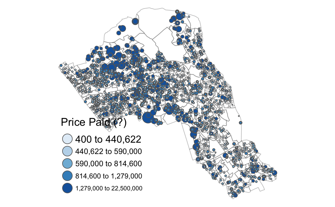

We can also make the polygon shapefile display one of our census variables as a choropleth map as shown below. In this example we have also added some more parameters within the tm_bubbles() function to create thin borders around the dots.

# creates a proportional symbol map
tm_shape(OA.Census) + 
  tm_fill("Qualification", palette = "Reds", style = "quantile", title = "% Qualification") +
  tm_borders(alpha=.4) +
  tm_shape(House.Points) + tm_bubbles(size = "Price", col = "Price", palette = "Blues", style = "quantile", legend.size.show = FALSE, title.col = "Price Paid (?)", border.col = "black", border.lwd = 0.1, border.alpha = 0.1) +
  tm_layout(legend.text.size = 0.8, legend.title.size = 1.1, frame = FALSE)
#> Some legend labels were too wide. These labels have been resized to 0.72. Increase legend.width (argument of tm_layout) to make the legend wider and therefore the labels larger.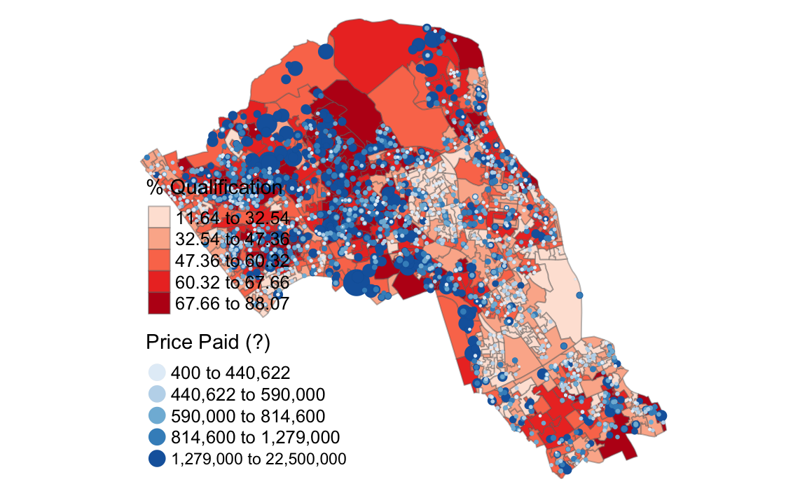

6.0.2.1 Saving the Shapefile

Finally, we can write the newly formed House.Points shapefile to our working directory

# write the shapefiel to your computer (remember to chang the dsn to your workspace)
writeOGR(House.Points, dsn = "worksheet_data/camden", layer = "Camden_house_sales", driver="ESRI Shapefile")

6.0.3 Final Task

Once you have completed the worksheet go to the data.police.uk website and click on the “Downloads” button. Download data for the Metropolitan Police for for the most recent July and also December. Open the files and extract only those rows that have an “LSOA name” containing Camden.

Produce a series of maps that show the distribution of crime for Camden: * How do crimes differ between July and December? * Do particular crime types appear to cluster together? * Are they related to demographic data? (when you create the spatialpointsdataframe you need to specify a different projection code. This is done as follows: proj4string = CRS(“+init=EPSG:4326”)